
Fick’s Laws
- Page ID
- 283250

Diffusion at the macroscopic scale: Fick’s equations
- Derivations come from the following book: Howard Berg, Random Walks in Biology, New and expanded edition, pp. 17 - 25.
- For students who need a review of 2nd derivatives and concavity, this link is helpful.
Fick’s laws describe the redistribution of particles in space over time. Rather than memorize them, it is useful to be able to derive them conceptually, starting from the rules of a random walk.
Fick’s first law: The motion of particles is driven by __________________________________.
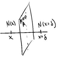
Let N(x) be the number of particles at position x, and N(x+δ) be the number of particles at position x+δ.
Let A be the area of the cross-sectional plane through which particles can pass [m2].
Let the time interval for motion be τ [s].
Define the flux, Jx, as the number of particles moving from left to right, per unit area of the cross-sectional plane, per unit time.
1a. Assume that all particles undergo a random walk. What fraction of the particles at position x move to the right in each time step?
1b. What fraction at position x+δ move to the left in each time step?
1c. Write an equation for the net number of particles that crosses to the right at each step:
1d. Write an equation for the net flux, Jx, in the x direction:
1e. What must be the units for flux, Jx?
1f. Recalling that the diffusion coefficient D = δ2/2τ, how could you manipulate the equation for J to have it include D? Tip: you need to multiply by a fraction (e.g. a/a) and rearrange.
1g. We would like to express flux in terms of concentration. Recalling that concentration C(x) is defined as the number of particles per unit volume, rewrite your equation for Jx in terms of C(x) instead of N(x).
1h. Here we need to recognize the definition of a derivative:
\[\dfrac{dy}{dx}=\underset{h→0}{\lim}\left(\dfrac{y(x+h)-y(x)}{h}\right)\nonumber\]
In the limit of very small δ, convert your equation (1g) to the derivative form of Fick’s first law:

NOTES:
Fick’s second law: Redistribution of particles over time is driven by ____________________________.
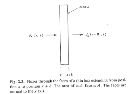
Consider particles moving through a volume whose cross-section is shown in the figure.
All particles follow a random walk.
We want to know how the concentration in the volume changes over time.
2a. Assume conservation of mass. What does this assumption mean about the particles?
2b. How many particles enter the volume from the left in a period of time, τ?
2c. How many leave out the right-hand face in this period?
2d. Calculate the change in concentration in this period:
2e. Calculate the change in C per unit time:
2f. In the limit of small τ and small δ, we have:
2g. Using Fick's first equation for Jx, we can rewrite this as Fick’s second law:
NOTES:
Contributors and Attributions
- Rebecca Pompano, University of Virginia (rrp2z@virginia.edu)
- Sourced from the Analytical Sciences Digital Library