Stationary Phase Mass Transport Broadening

Consider a compound that has distributed between the mobile and stationary phase within a plate in a chromatographic column. Figure 27 might represent the concentration distribution profiles in the two phases (note that the compound, as depicted, has a slight preference for the mobile phase).

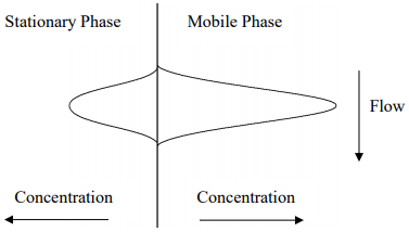
Figure 27. Representation of the concentration profiles for a compound distributed between the stationary (left) and mobile (right) phases of a chromatographic column. Note that the compound has a preference for the mobile phase.

What we want to do is consider what would happen to these two concentration profiles a brief instant of time later. Since the mobile phase is mobile and the solute molecules in it are moving, we could anticipate that the profile for the mobile phase would move ahead a small amount. The figure below illustrates this.

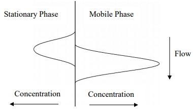
Figure 28. Representation of the two concentrations profiles in Figure 27 a brief instant of time later. Note that the mobile phase profile has moved ahead of the stationary phase profile.

What about the concentration profile for the solute molecules in the stationary phase? Consider the picture in Figure 29 for two solute molecules dissolved in the stationary phase of a capillary column and let’s assume that these are at the trailing edge of the stationary phase distribution.

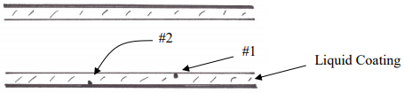
Figure 29. Two molecules dissolved in the liquid stationary phase of a capillary column.

What we observe is that the molecule labeled 1 is right at the interface between the stationary and mobile phase and provided it is diffusing in the right direction, it can transfer out into the mobile phase and move along. The molecule labeled 2, however, is “trapped” in the stationary phase. It cannot get out into the mobile phase until it first diffuses up to the interface. We refer to this process as mass transport. The solute molecules in the stationary phase must be transported up to the interface before they can switch phases. What we observe is that the solute molecules must spend a finite amount of time in the stationary phase. Since the mobile phase solute molecules are moving away, molecules stuck in the stationary phase lag behind and introduce a degree of broadening.

If we then consider the leading edge of the mobile phase distribution, we would observe that the molecules are encountering fresh stationary phase with no dissolved solute molecules and so these start to diffuse into the stationary phase when they encounter the surface. We can illustrate this in Figure 30 with arrows showing the direction of migration of solute molecules out of the stationary phase at the trailing edge and into the stationary phase at the leading edge.

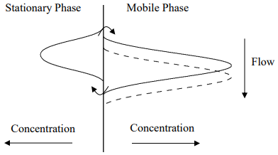
Figure 30. Representation of the movement of analyte molecules at the leading and trailing edge of the concentration distribution.

Hopefully it is obvious from Figure 30 that the finite time required for the molecules to move out of the stationary phase leads to an overall broadening of the concentration distribution and overall broadening of the peak.

A critical question to ask is whether the contribution of stationary phase mass transport broadening exhibits a dependence on the flow rate. Suppose we go back to the small amount of time in the first part above, but now double the flow rate. Comparing the first situation (solid line in the figure above) to that with double the flow rate (dashed line) leads to the two profiles. Hopefully it is apparent that the higher flow rate leads to a greater discrepancy between the mobile and stationary phase concentration distributions, which would lead to more broadening.

The term used to express mass transport broadening in the stationary phase is C_S (not to be confused with the C_S that we have been using earlier to denote the concentration of solute in the stationary phase). If we wanted to incorporate this into our overall band broadening equation, recognizing that higher flow rates lead to more mass transport broadening and reduced column efficiency (higher values of h), it would take the following form:

\[\mathrm{h = C_S\, v}\]

Something we might ask is whether the flow rate dependency of the stationary phase mass transport term has any troublesome aspects. An alternative way to phrase this question is to ask whether we would like to use slow or fast flow rates when performing chromatographic separations. The advantage of fast flow rates is that the chromatographic separation will take place in a shorter time. Since “time is money”, shorter analysis times are preferred (unless you like to read long novels, and so prefer to inject a sample and then have an hour of reading time while the compounds wend their way through the column). If you work for Wenzel Analytical, we’re going to try to perform analyses as fast as possible and maximize our throughput. The problem with speeding up the flow rate too high is that we begin to introduce large amounts of stationary phase mass transport broadening. The shortening of the analysis time begins to be offset by broad peaks that are not fully separated. Ultimately, stationary phase mass transport broadening forces us to make a compromise between adequate efficiency and analysis time. You cannot optimize both at the same time.

Another thing we need to think about is what effect the thickness of the stationary phase has on the magnitude of stationary phase mass transport broadening. The pictures in Figure 31 for one wall of a coated capillary column serve to illustrate this point.

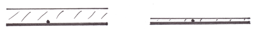
Figure 31. Representation for one wall of a coated capillary column with a thicker (left) and thinner (right) stationary phase coating.

Remember that the key point is that solute molecules spend a finite amount of time in the stationary phase, and since solute molecules in the mobile phase are moving away, the longer this finite time the worse. Therefore the thicker the phase, the more broadening will occur from stationary phase mass transport processes. This says that the ideal stationary phase coating ought to be microscopically thin, so that molecules rapidly diffuse into and out of the stationary phase, thereby reducing how far ahead mobile phase molecules can move in this finite amount of time. We should also be able to realize that the optimal coated phase ought to have a uniform thickness. If we have thin and thick regions as shown in Figure 32, we see that the time spent in the stationary phase by solute molecules will vary considerably, an undesirable situation. Compound 1 will likely spend less time in the stationary phase than compound 2.

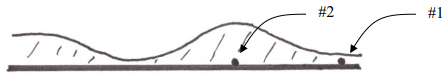
Figure 32. Representation of one wall of a coated capillary column with non-uniform thickness of the coating.

While microscopically thin coatings reduce stationary phase mass transport broadening, there are two problems with microscopically thin coated phases. If we consider the picture in Figure 31, where we have two capillary columns with different thickness coatings, the capillary column with the thinner coating will have much lower capacity than the one with the thicker coating. This means that there is much less weight of stationary phase over a theoretical plate for the column with the thinner coating and much less analyte dissolves into the stationary phase. Increasing the thickness of the coating or capacity of the column has several advantages. One is that it helps in the separation of the mixture (something we will learn more about later in the course). The other is that it is easy to overload or saturate a column that has a very low capacity.

This raises the question of whether you could design a column that has a thin stationary phase coating but high capacity. For coated capillary columns, this is not possible. A thinner coating in a capillary column means less capacity. For a coated packed column; however, it is possible to retain a high capacity while thinning the coating. Accomplishing this involves using smaller particles but the same weight of coating. Imagine taking large solid support particles and crushing them into a bunch of smaller particles. What you should realize is that the smaller particles have a much larger surface area. If we then coated the same amount of stationary phase (e.g., 5% by weight) relative to the weight of solid support, because of the larger surface area a thinner coating results. What we see is that the use of smaller particles has a theoretical advantage over the use of larger particles for coated stationary phases.

Another problem with coating microscopically thin phases is the risk of leaving some of the surface of the underlying solid support uncoated. These exposed solid surfaces (Figure 33) provide highly active sites for adsorption of solute molecules, and we have already seen how adsorption is an inefficient process that leads to peak tailing. While thin coatings have an advantage, great care must be taken in coating these phases to insure a complete coverage with uniform thickness of the surface.

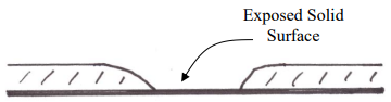
Figure 33. Representation of the wall of a coated capillary column showing an exposed solid surface.

Open tubular capillary columns are common in gas chromatography because it is possible to coat their inside walls with an exceptionally thin, uniform stationary phase. Today, it is also possible to chemically bond the liquid phase onto the interior surface of the capillary column. In the early days of capillary gas chromatographic columns, these were made of glass tubing that was approximately the same diameter as a melting point capillary that you are familiar with from organic chemistry. These columns were stretched from thick-walled glass tubes that were heated in an oven. As the capillary tube was stretched out, it was coiled in a coiling oven. It was common to use 30-meter lengths, essentially a 30-meter long glass slinky. The most common process for coating a capillary column involves what is known as the “moving plug” technique. As illustrated in Figure 34, the liquid stationary phase is dissolved in a plug of solvent that is pushed through the column using pressure from an inert gas. As the plug moves, it coats a very thin layer of liquid onto the inside walls of the column. As the solvent evaporates, a very thin layer of liquid stationary phase remains on the walls of the column. A systematic process is used to treat the inside walls of the column prior to coating to ensure that the liquid wets the surface well and is deposited uniformly over all of the interior surfaces.

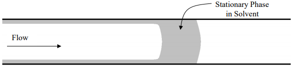
Figure 34. Moving plug technique for coating a capillary column.

One problem with these glass columns was their fragility. Many frustrated workers broke the columns trying to mount them into a gas chromatograph with leak-proof fittings. The fittings used with these glass columns are usually made of graphite, a soft substance that often can be molded around the tube without breaking it (but if you’re not careful, it’s easy to break it). Another problem is caused by the chemical nature of glass. We think of glass as a silicate material (SiO₂), but it actually turns out that most silicate glasses contain other metal ions as constituents (aluminum, magnesium, calcium, and iron oxides are some of the other metals present). In some glasses, these other metals can be as much as 50% of the glass. These metals are positively charged centers, and if some of the surfaces are not coated by the liquid phase (an inevitable occurrence), these metal ions provide active sites for adsorption that cause tailing of compounds (especially oxygen- and nitrogen-containing compounds that have dipoles).

The capillary columns used in gas chromatography today are known as fused silica columns. Fused silica is pure silicon dioxide (SiO₂) and lacks the metal ions in regular glass. The surface of fused silica is considerably less active than the surface of regular glass. Fused silica is widely used in the production of devices known as fiber optics. Fiber optics are thin, solid glass fibers. Light is shined into one end of the fiber at an angle that causes complete internal reflection of the light as shown in Figure 35.

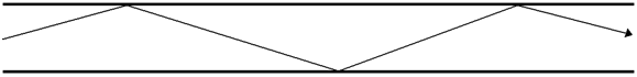
Figure 35. Complete internal reflection of a light beam inside a fiber optic.

Light going in one end (e.g., New York City) exits out the other end (e.g., Los Angeles, CA). The light can be pulsed (sent in small bursts) and the speed of light allows for very rapid communication. It turns out to be easy to make fiber optic-like devices with a hole in the center (in fact, it took people a while to learn how to make glass fibers without the hole since the fibers tend to cool from the outside to the inside, leading to contraction and a hole in the center). The hole in the center of fused silica capillary columns is so small you cannot see it with the naked eye (we will see later that this very small opening has advantages in chromatographic applications). Also, these capillary columns are incredibly flexible. They can be tied into knots, and more importantly for chromatographic applications, leak-tight fittings can be attached without breaking the columns. The deactivated surface, flexible nature making them easy to install and use, and chromatographic efficiency (partly because of the deactivated surface, partly because of how well they can be coated with thin phases, and partly because of the small diameter) make them the column of choice for most gas chromatographic applications today. The only drawback to these columns is that they have very small capacities. Gas chromatographs built to use fused silica capillary columns usually have what are known as split injection systems. A typical injection size for a gas chromatographic sample is 1 µL. Even this amount is too much for a fused silica capillary column, but reproducibly injecting smaller volumes is very difficult. Instead, the flow from the injector is split, and only a small part (often 1 in 50 to 1 in 100) is actually sent into the capillary column. The rest is vented away and never enters the column.

Another thing we need to examine under the topic of stationary phase mass transport broadening is the nature of the stationary phase used today in liquid chromatography. In 1963, Calvin Giddings published a significant paper titled “Liquid Chromatography with Operating Conditions Analogous to Those of Gas Chromatography” (Analytical Chemistry, 1963, 25, 2215). At this point in time, gas chromatography was the method of choice when performing analyses because existing gas chromatographic columns were far more efficient than the liquid chromatographic columns that were available. In fact, gas chromatography was so preferable to liquid chromatography that many publications of the 1960s and 1970s described ways of preparing volatile derivatives of non-volatile compounds so that they could be analyzed by gas chromatography. The extra steps involved in the derivatization were worthwhile since liquid chromatographic methods were not good enough to separate most compounds in complex mixtures.

What Giddings did in this paper was show that it was theoretically possible to perform liquid chromatography at the efficiency of gas chromatography. The key feature, which we have not yet fully developed because we have one more contribution to broadening to examine, was to use exceptionally small particles with exceptionally thin coatings in liquid chromatographic columns. Of course, these exceptionally thin coatings cause several problems. One is how to coat them so that none of the surface of the solid support is exposed. If you can coat them uniformly, another problem in a liquid chromatographic system is that there might be locations in the column where the flowing liquid mobile phase can physically wash away regions of the coated phase thereby exposing the underlying solid surface. Finally, there is no such thing as two liquids that are completely immiscible in each other. It’s true that oil and water don’t mix, but it’s also true that a little bit of oil will dissolve in water. Over time, the coated stationary phase will gradually dissolve away in the mobile phase, eventually exposing the underlying solid surface. Even though Giddings showed in 1963 how to perform liquid chromatography at the efficiency of gas chromatography, the phases that were needed could not be coated in a way that it was a widely practical method.

It was not until the late 1970s, when bonded liquid chromatographic stationary phases were introduced, that it was finally practical to do liquid chromatography with the same efficiency as gas chromatography. Bonded phases relied on silica gel, something we already encountered when we first talked about solid phase, adsorption chromatography. Silica gel is an excellent support for liquid chromatographic phases. It is physically robust, stable at pH values from about 2 to 8, and can be synthesized in a range of particle sizes including the very small particle sizes needed for liquid chromatography. The chemistry used in preparing bonded phases is shown in Figure 36. Basically this involves the surface derivatization of the silanol groups on the surface of the silica gel with chlorodimethyloctadecylsilane. The C₁₈ or octadecylsilane (ODS) phase shown in the scheme are the most common ones used. The pyridine is added to remove the HCl produced in the reaction.

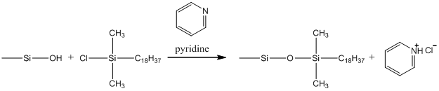
Figure 36. Scheme for bonding C₁₈ groups to the surface of silica gel.

Other common bonded phases use C₈ or C₁ surface groups. You can also purchase bonded phases with phenyl groups, C₃H₆NH₂ (aminopropyl) groups, and C₃H₆CN groups. But the C₁₈ phases are so common, and so versatile, that we will examine these in more detail.

The first thing to realize is that attaching the C₁₈ groups converts a highly polar surface (the silanol groups can form hydrogen bonds) into a non-polar surface. In effect, this is like attaching a one-molecule thick, oily skin to the surface of silica gel. There is some question about the exact conformation of the attached C₁₈ groups. Figure 37 shows two forms, one with the C₁₈ groups extended, the other with the C₁₈ groups collapsed. There is substantial evidence to support the idea that if the non-polar C₁₈ phase is in contact with a mobile phase that is very polar (e.g., water), that the C₁₈ groups are in the collapsed form. Putting the C₁₈ phase in contact with a less polar mobile phase (e.g, methanol) leads to more extension of the C₁₈ groups.

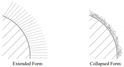
Figure 37. Extended and collapsed forms of C₁₈ groups bonded to the surface of silica gel.

If we examine the extended form of the C₁₈ phase, it is interesting to consider the nature of this material at the outer regions. Even though the C₁₈ groups are attached to a solid, are they long enough such that the outer edges are “fluid” enough to behave more like a liquid than a solid? If so, then molecules might distribute into these phases by a partitioning mechanism. If not, then molecules adsorb to the surface. We previously learned that adsorption was undesirable when compared to partitioning, but that was adsorption on a polar surface. The non-polar, deactivated nature of the C₁₈ surface does not provide strong adsorption sites so peak tailing is quite minimal with C₁₈ bonded phases.

If you look at most liquid chromatograms, though, you will see that the peaks tail more than in gas chromatography. The likely reason for this is that some of the surface silanol groups remain underivatized. Crowding of the C₁₈ groups during the derivatization process makes it unlikely that all of the silanols can be reached and deactivated. In an effort to minimize the number of unreacted silanol groups, some commercially available C₁₈ phases are end-capped. End capping involves exhaustively reacting the C₁₈ phase with a much smaller silane such as chlorotrimethylsilane (ClSi(CH₃)₃).

Because of the covalent bonds, the C₁₈ groups cannot wash or dissolve off of the solid support. With regards to mass transport in the stationary phase, we said that we want the stationary phase as thin as possible. C₁₈ bonded phases are essentially one-molecule thick. We could never coat a one-molecule thick chromatographic phase that was uniform and had no exposed solid surfaces. Therefore, we could never really make a liquid chromatographic phase with faster stationary phase mass transport properties than the bonded silica phases.

Until recently, the common particle sizes to find in commercially available C₁₈ columns had diameters of 3, 5, and 10 µm. Columns using particles of these sizes are commonly referred to as high performance liquid chromatography (HPLC). Recently columns with 1.7 or 1.8 um particles have become commercially available and there use is referred to as ultra-high pressure liquid chromatography (UPLC). Smaller particles will require higher pressures to force a liquid through the column and UPLC columns can run at pressures up to 15,000 psi. In gas chromatography, we observe that smaller particles usually have thinner coatings because they have more surface area. Note that for these bonded phases the thickness of the stationary phase with the 1.7, 3, 5, and 10 µm particles is always identical. What does change is the surface area. A column packed with 3 µm particles will have more surface area than a column of the same length packed with 5 or 10 µm particles. This increased surface area leads to an increase in the column’s capacity. If the columns are the same length, the increased capacity will lead to increased separation of compounds and lengthen the retention times. The usual approach is to use shorter columns with the smaller particles. The shorter column reduces the analysis time because there is less volume of mobile phase in the column. Typically C₁₈ columns packed with 10 µm particles are 25 cm long; 5 µm particles are used in columns that are 15 cm long; and 3 µm particles are used in columns that are 3 cm long. These 3×3 columns can have very short analysis times. A negative aspect is that they are more susceptible to fouling by contaminants in the sample. Also, a difficulty with ultra-small particles involves packing the columns so that there are no channels. Because of the small particles, liquid chromatographic columns require highly specialized packing procedures. Finally, the particles need to have uniform sizes (the smaller the particle, the smaller the tolerance on the range of particle sizes that can be used). A mixture of particles of different sizes is known as an aggregate. Concrete is an excellent example of an aggregate. The problem with an aggregate is that the smaller particles fill in the voids between the larger particles, making it very difficult to get a liquid to flow through the bed.

One last thing we can consider is whether stationary phase mass transport broadening is more significant in gas or liquid chromatography. We have to be careful here, because it’s a somewhat subtle distinction. What we need to consider is the diffusion rate of the solute in the stationary phase. In gas chromatography, we have a gaseous molecule dissolved in a liquid coating. The important thing is that it is a dense liquid with a molecule dissolved in it. The diffusion rate is therefore rather comparable in this stationary phase to that of a liquid. Of course, a liquid chromatographic column is usually at room temperature whereas a gas chromatographic column is usually at some elevated temperature that is often higher than 100^oC. We know that diffusion rates are temperature dependent, so that the rate ought to be faster in gas chromatography, and mass transport broadening in the stationary phase ought to be more significant in liquid chromatography, assuming everything else is equal. Just realize that this is not a 100,000-fold difference, because the stationary phase in gas chromatography is not a gas, but a heated liquid. It is also possible to operate liquid chromatographic columns at higher temperatures to speed up the rate of diffusion and improve the mass-transport broadening.