Classical Description of NMR Spectroscopy

The quantum mechanical description developed in the preceding section of this unit is useful in understanding many important concepts of NMR spectroscopy. However, to understand how the spectrum is obtained on the types of instruments in use today, it is necessary to consider what is known as the classical description of NMR spectroscopy. Earlier we mentioned that the ground spin state of a proton is one in which its magnetic field is aligned “with” B_APPL. In actuality, there is a subtlety to the motion of the hydrogen nucleus that we have not considered yet. The diagram in Figure 26 will help understand the actual motion that occurs. Note that the diagram in Figure 26 also places the spinning proton on a coordinate system. A coordinate system is needed because magnetic fields have a direction to them. The external applied magnetic field in an NMR spectrometer is usually considered to be on the Z-axis.

As shown in Figure 26, the actual magnetization vector (B_P) created on the axis of spin of the hydrogen nucleus is not perfectly aligned with B_APPL but instead is tipped a bit off from B_APPL. What also happens in addition to the spinning motion of the proton is that its magnetization vector precesses about B_APPL. The precessional motion effectively transcribes a cone shape as shown in Figure 26. Note that the precessional motion for the ¹H nucleus depicted in Figure 26 is opposite (clockwise) to the spinning motion (counterclockwise).

An important consideration is that there is a large ensemble of nuclei that are in the many molecules in the NMR tube. Of this ensemble, we know that a slight excess are in the ground state with their magnetic field aligned “with” B_APPL. So Figure 26 effectively shows the vector representations for the excess nuclei in the ground state. It is also important to recognize that this ensemble of many nuclei do not precess in phase with each other. For every nucleus that at some moment has a +X or +Y component of magnetization, there is a corresponding nucleus that at the same moment has a –X or –Y component of magnetization. The result is that the X and Y components of the magnetization cancel out over the entire ensemble of nuclei and the only finite component of magnetization is along the Z-axis. Hence, the net magnetization vector lies only on the Z-axis as shown in Figure 26.

Figure 26. Movement of the spinning proton showing that its nuclear magnetic dipole does not align with B_APPL but is slightly off axis and precesses about B_APPL.

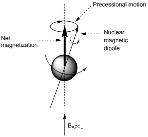
There are two things to consider about this precessional motion. Imagine yourself sitting on top of the proton’s magnetization vector as it precessed about B_APPL. You would have a certain precessional speed or a precessional velocity. Furthermore, as you precess about around B_APPL you could count how many cycles you made in a second. This would be your precessional frequency, which is also known as the Larmor frequency. The relationship that describes the precessional or Larmor frequency of a nucleus is shown in Eq 11. An important outcome is to recognize that Eq 11 for the precessional frequency in the classical description of NMR spectroscopy is identical to Eq 4 obtained in the quantum mechanical description of NMR spectroscopy.

\[v = \dfrac{uB_o}{hI} \tag{11}\]

What the classical description allows us to better understand is what happens to the nucleus when it is excited and how signal is measured on today’s instruments. When examining pictures of what occurs with a nucleus in the NMR spectrometer, two things are important to consider. One that has already been mentioned is that there is a large ensemble of nuclei that are in the many molecules in the NMR tube, and we are examining the excess within this ensemble that have their magnetic field aligned “with” B_APPL. The other is that it helps to examine pictures of the behavior of a nucleus by operating in what is known as the rotating frame. Operating in the rotating frame means that the observer is rotating at the same rate that the nucleus being examined is precessing. The result is that, instead of observing individual vectors precessing about B_APPL, only the net magnetization vector is observed. Figure 26 also shows a vector representing the net magnetization for an observer in the rotating frame. Note that the net magnetization is effectively a time average of the nuclear magnetic dipole of the precessing nucleus.

A design feature of NMR spectrometers is to place a coil of wire on the X-axis. An electrical current that oscillates at a radiofrequency is then run through the coil.

What happens when an electrical current is run through a wire coil?

It turns out that running an electrical current through a wire coil generates a magnetic field (designated B₁) as shown in Figure 27. Note that B₁ is oriented perpendicular to B_APPL.

Figure 27. Representation of B₁, which is produced by the RF coil, and the torqueing of the net magnetization vector for the proton that occurs when the frequency used to generate B₁ exactly matches the precessional frequency of the proton.

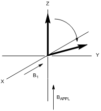
Let’s consider a compound whose NMR spectrum consists only of a singlet (e.g., tetramethylsilane) so there is only one excitation frequency. If the current of electricity used to generate B₁ oscillates at a frequency that exactly corresponds to the precessional frequency of the nucleus responsible for the singlet, B₁ exerts a torque (or force) on that nucleus with the result that the nucleus now wants to precess about B₁ instead of B_APPL. Looking only at the net magnetization vector in Figure 27, when a matching B₁ is applied the nucleus tips off the Z-axis in the Y-Z plane as it begins to precess about B₁.

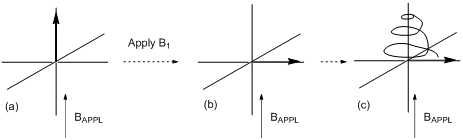
When recording an NMR spectrum, B₁ is only applied for a few microseconds (this brief application of B₁ is referred to as a pulse). Suppose B₁ is applied just long enough to tip the net magnetization vector of the proton by 90^o as shown in Figure 28b and is then turned off. Note: the extent to which nuclei tip is directly dependent on the length of the RF pulse. If 10 usec resulted in a 90^o tip, 5 usec would result in a 45^o tip.

Figure 28. Representation of what happens to the net magnetization vector after (b) application of a 90^o pulse. B₁ is turned on for a short period of time to tip the vector. After turning off the vector, the nucleus undergoes a “spiral-like” motion (c) as it returns to its normal precessional motion about BAPPL.

What happens to the nucleus after B₁ is turned off?

The nucleus now needs to precess about B_APPL but it starts the precession with its magnetization vector located in the X-Y plane. It will gradually relax back because of spin-lattice (longitudinal) relaxation in a spiral-like motion to its starting state finally forming a precessional cone about B_APPL as shown in Figure 28.

Remember that the diagrams in Figure 28 represent those of an ensemble of nuclei tipped during the RF pulse. In their original precessional motion, the nuclei were out of phase with each other. When the nuclei are tipped, the net magnetization of each is in phase on the Y-axis. While spin-lattice relaxation is responsible for the spiraling relaxation illustrated in Figure 28, spin-spin (transverse) relaxation results in ground and excited state nuclei swapping states. Newly excited nuclei formed through this spin-spin process are no longer in phase with the other excited nuclei. This dephasing of the nuclei through spin-spin relaxation will lead to a reduction of the recorded signal.

Suppose a wire coil is placed on the Y-axis. What happens in the wire coil as the magnetic field of the tipped nucleus is imparted on it?

Applying a magnetic field to a wire coil will generate an electrical current. In reality, instead of having a second wire coil on the Y-axis, the wire coil on the X-axis is used. In the first step, an RF pulse is applied through the coil to excite or tip the nucleus. Once the pulse is turned off, the coil can be used to measure the electric current generated by the magnetic field of the tipped nucleus.

Draw the current profile that would result in the wire coil on the X-axis as the tipped nucleus relaxes back to its ground state.

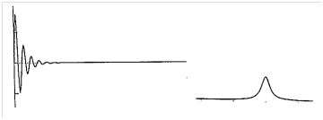
As the nucleus precesses around B_APPL during the relaxation process, it has alternating positive and negative components of magnetization on the X-axis. The result is the current profile shown in Figure 29a. This profile is referred to as a free induction decay (FID). The FID is a representation of the resonance of the single nucleus being excited, but it is in what is called the time domain. A mathematical technique called a Fourier transform (FT) can be used to analyze a wave form and determine the individual frequency components and their amplitudes that are needed to generate the wave. The outcome of performing an FT on an FID yields what is called the frequency domain spectrum, which is shown in Figure 29b. This is the common spectrum we see in NMR spectroscopy with the amplitude of peaks on the Y-axis and resonances reported in ppm on the X-axis.

Figure 29. (a) Free induction decay (FID) for a nucleus with a single precessional frequency. The FID is known as the time-domain spectrum. (b) The frequency domain spectrum, which is a singlet, obtained by performing a Fourier transform of the FID.

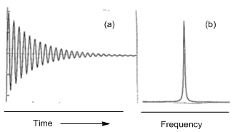
In drawing the FID in Figure 29a, it might be tempting to think of each positive and negative component of the FID representing the magnetic vector of the nucleus as it is positioned on the +X and –X axis. A problem with this thinking is to consider a specific ¹H resonance occurring at 400 MHz, as we have been using in some of our examples. The vector actually oscillates between the +X and –X direction 400 million times a second, which would mean that the FID shown in Figure 29a should have 400 million oscillations in a second. This would be incredibly challenging to measure. We will not develop the details of how the measurement of the FID is actually obtained, but there is an electronic process that can be used in which the FID shows the difference in frequencies between the peaks in the spectrum and what is known as the carrier frequency. What we will see is that, when recording NMR spectra, rather than applying a single RF frequency through the wire coil on the X-axis, the instrument applies a broadband pulse of radiofrequencies that can excite all of the hydrogen nuclei at once. The carrier frequency is the center frequency of the broadband RF pulse that is applied. These differences are only on the order of a few thousand Hertz. Oscillations of a few thousand times a second are readily measured using modern digital electronics.

Draw the FID that would result if the nucleus had a much shorter relaxation time.

With a shorter relaxation time, the decay of the FID would be must faster. The FID for a nucleus of identical excitation frequency to that in Figure 29 but with a much shorter relaxation time is shown in Figures 30.

Figure 30. The FID (left-hand side) of a nucleus with the same excitation frequency as that in Figure 29 but a much shorter relaxation time. The frequency domain spectrum (right-hand side) that arises out of performing the Fourier transform of the FID. Note that the frequency domain spectrum in Figure 30 is a much broader singlet than occurs in Figure 29.

Do you see a problem with performing a FT on an FID with a very short relaxation time? If so, what would happen in the resulting frequency domain spectrum?

It will be more difficult to identify the frequency of the highly truncated FID with as much accuracy as an FID with a much slower decay. The difficulty in determining an exact frequency means that the resonance will be much broader in the frequency domain spectrum as shown in Figure 30. An outcome of the signal decay in an FID means that every peak in the frequency domain spectrum will have some amount of broadening, and the faster decay the more the broadening.

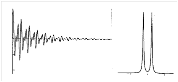
As mentioned previously, rather than applying a single RF frequency through the wire coil on the X-axis, the instrument applies a broadband pulse of radiofrequencies that can excite all of the hydrogen nuclei at once. Suppose we consider a sample whose spectrum consists of two singlets with slightly different excitation frequencies. If both are excited at once through the broadband RF pulse, the FID will consist of a composite wave that is the sum of the two contributing components as shown on the left in Figure 31. The FT can determine the frequency components and their amplitude of both contributing waves in the composite time domain wave and generate the corresponding frequency domain spectrum shown on the right in Figure 31.

Figure 31. The left-hand side is the FID of a sample where the NMR spectrum consists of two singlets of slightly different frequency. The right-hand side is the frequency domain spectrum showing the two singlets that arises out of performing the Fourier transform of the FID.

Where is the amplitude of peaks determined in the FID?

Because of the decay and the fact that different nuclei in a molecule will have different decay rates, the amplitude of each peak must be determined using the first data point in the FID.

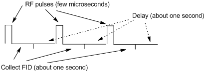
The typical pulse sequence used when recording standard ¹H NMR spectra is shown in Figure 32. A brief (few microsecond) broadband RF pulse is applied to tip the net magnetization of all the nuclei, the X-coil is turned on to sample the FID (about 1 second) and then there is a delay time (about 1 second). Then the sequence is repeated multiple times and the FIDs are added together.

Figure 32. Diagram of the normal pulse sequence for collecting NMR spectra that involves a brief RF pulse, sampling of data to collect the FID, and a delay time.

Why is a delay time incorporated into the sequence?

The purpose of the delay time is to allow more complete relaxation of the nuclei. If the nuclei are not allowed to relax back to the ground state, the transition may become saturated and then there will be no signal to record.

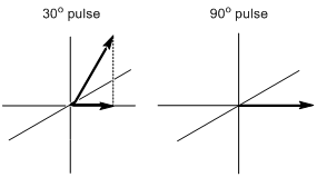
So far we have developed our understanding of FT NMR using 90^o pulses. In reality, 90^o pulses are rarely used when obtaining routine spectra and the use of 30^o pulses is more common.

Why are the advantages and disadvantages of using 30^o pulses instead of 90^o pulses?

As seen in Figure 33, if only a one pulse measurement is performed, a disadvantage of using a 30^o pulse instead of a 90^o pulse is that there is a smaller magnetization on the X-Y axes and less amplitude in the FID. That means that the signal-to-noise ratio will be smaller for the 30^o pulse. However, NMR spectra are rarely recorded using a single pulse. Instead, several repetitive pulses using the sequence in Figure 32 are run and added together. The advantage of the 30^o pulse over the 90^o pulse is that it better insures that the nuclei have relaxed back to the ground state after each pulse so that resonances are less likely to get saturated. Clearly this is a tradeoff and whether to use a 30^o pulse or 90^o pulse can depend on the particular relaxation times of nuclei in the sample.

Figure 33. Comparison of 30^o and 90^o pulses. Note how there is much less x-component of magnetization with the 30^o pulse.

What is the advantage of recording several FIDs and adding them together?

As mentioned earlier in this unit, signal is consistent from run to run but noise is random. Adding several FIDs together leads to some cancelling out of the noise but growth of the signal, thereby improving the S/N ratio.

One final thing to consider is the behavior of a nucleus with a very long spin-lattice relaxation time. ¹³C is a spin ½ nucleus and it is possible to obtain ¹³C NMR spectra. The primary mode of relaxation of ¹³C atoms is through an interaction with the nucleus of directly bonded hydrogen atoms. Carbon atoms in a compound with no directly bonded hydrogen atoms (e.g., tertiary carbon atoms, substituted aromatic carbon atoms, carbonyl carbon atoms in a ketone) can have very long relaxation times – upwards of 100 seconds.

Suppose the following pulse sequence is used to obtain the spectrum of a ¹³C nucleus with a spin-lattice relaxation time of 100 seconds (90^o pulse, 1 second collection of the FID, 1 second delay). Note, carbon atoms with no directly bonded hydrogen atoms can have relaxation times as long as 100 seconds. This pulse sequence is repeated four times.

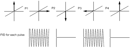
• Draw the position of the ¹³C magnetization vector after each of the four pulses.
• Draw the corresponding FID that would be obtained after each pulse.
• Draw the composite FID obtained by adding the four individual FIDs together.
• What do you observe for this carbon in the resulting frequency domain spectrum?

The important point to consider is that the ¹³C nucleus in question has almost no relaxation between each pulse. This means that the second pulse will put its net magnetization vector on the –Z axis as shown in Figure 34. The third pulse puts the net magnetization vector on the –Y axis, and the fourth pulse puts the vector back where it originally started. For pulses 2 and 4, there is no net magnetization in the XY plane so there is no signal recorded in the FID. For pulses 1 and 3, there is a net magnetization in the XY plane, but the two FIDs are exactly out of phase with each other (out of phase means that where one of the FIDs has a positive amplitude, the other has the exact same amplitude but negative) (Figure 34). Adding these four together gives a net result of no FID for this nucleus. That means that the resulting frequency domain NMR spectrum will show no peak for this carbon. What we would also say about this carbon is that we have saturated the transition.

Figure 34. Top: net magnetization vector for four consecutive 90^o pulses for a nucleus with an exceptionally long relaxation time. Bottom: corresponding FID for each of the four pulses.

The influence of saturation on atoms with different relaxation times is exploited in the technique magnetic resonance imaging (MRI). MRI is used to generate high quality images in humans. The signal recorded in MRI is the hydrogen resonance of water molecules. A paramagnetic complex of gadolinium(III) is often used as an image contrast agent and is consumed ahead of time by the person having the MRI. Paramagnetic substances promote nuclear relaxation so greatly shorten the relaxation times of the hydrogen atoms in water. But the paramagnetic gadolinium complex distributes differently into different tissues in the body. For example, in a cancerous brain tumor, a higher concentration of gadolinium goes into the tumor than into the surrounding tissue. That means the relaxation time of hydrogen atoms in the water in the tumor is shorter than the relaxation time of hydrogen atoms in the water outside the tumor. By carefully setting up the pulse sequence, it is possible to observe signal for water molecules inside the tumor that have faster relaxation while saturating and observing minimal signal for water molecules outside the tumor because of their slower relaxation. The ability to record NMR spectra of humans is so significant advance that it resulted in a Nobel Prize for those individuals most responsible for inventing the method.