
3.6: Variables that Influence Fluorescence Measurements
- Page ID
- 111568

What variables influence fluorescence measurements? For each variable, describe its relationship to the intensity of fluorescence emission.
There are a variety of variables that influence the signal observed in fluorescence spectroscopy. As seen in the original diagram showing the various energy levels and transitions that can occur, anything that can quench the fluorescent transition will affect the intensity of the fluorescence.
When discussing absorption spectroscopy, an important consideration is Beer’s Law. A similar relationship exists for fluorescence spectroscopy, as shown below, in which \(I\) is the fluorescence intensity, \(\varepsilon\) is the molar absorptivity, \(b\) is the path length, \(c\) is the concentration, and \(P_o\) is the source power.
\[\mathrm{I = 2.303K’\varepsilon bcP_o} \nonumber \]
Not surprisingly, fluorescence intensity varies linearly with the path length and with the concentration. K’ is a constant that is dependent on the geometry and other factors and includes the fluorescence quantum yield. Since \(\varphi_F\) is a constant for a given system, K’ is defined as K”\(\varphi\)F. Of particular interest is that the fluorescence intensity relates directly to the source power. It stands to reason that the higher the source power, the more species that absorb photons and become excited, and therefore the more that eventually emit fluorescence radiation. This suggests that high-powered lasers, provided they emit at the proper wavelength of radiation to excite a system, have the potential to be excellent sources for fluorescence spectroscopy.
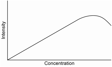
The equation above predicts a linear relationship between fluorescence intensity and concentration. However, the utility of this equation breaks down at absorbance values of 0.05 or higher leading to a negative deviation of the standard curve.
Something else that can possibly occur with fluorescence or other emission processes is that emitted photons can be reabsorbed by ground state molecules. This is a particular problem if the S1-S0 emission transition is the one being monitored. In this situation, at high concentrations of analyte, the fluorescence intensity measured at the detector may actually start to drop as shown in the standard curve in Figure \(\PageIndex{8}\).
Any changes in the system that will affect the number and force of collisions taking place in the solution will influence the magnitude of the fluorescence emission. Collisions promote radiationless decay and loss of extra energy as heat, so more collisions or more forceful collisions will promote radiationless decay and reduce fluorescence emission. Therefore, fluorescent intensity is dependent on the temperature of the solution. Higher temperatures will speed up the movement of the molecules (i.e., higher translational energy) leading to more collisions and more forceful collisions, thereby reducing the fluorescent intensity. Insuring that all the measurements are done at the same temperature is important. Reducing the temperature of the sample will also increase the signal-to-noise ratio.
Another factor that will affect the number of collisions is the solvent viscosity. More viscous solutions will have fewer collisions, less collisional deactivation, and higher fluorescent intensity.
The solvent can have other effects as well, similar to what we previously discussed in the section on UV/VIS absorption spectroscopy. For example, a hydrogen-bonding solvent can influence the value of \(\lambda\)max in the excitation and emission spectra by altering the energy levels of non-bonding electrons and electrons in \(\pi\)* orbitals. Other species in the solution (e.g., metal ions) may also associate with the analyte and change the \(\lambda\)max values.
Many metal ions and dissolved oxygen are paramagnetic. We already mentioned that paramagnetic species promote intersystem crossing, thereby quenching the fluorescence. Removal of paramagnetic metal ions from a sample is not necessarily a trivial matter. Removing dissolved oxygen gas is easily done by purging the sample with a diamagnetic, inert gas such as nitrogen, argon or helium. All solution-phase samples should be purged of oxygen gas prior to the analysis.
Another concern that can distinguish sample solutions from the blank and standards is the possibility that the unknown solutions have impurities that can absorb the fluorescent emission from the analyte. Comparing the fluorescent excitation and emission spectra of the unknown samples to the standards may provide an indication of whether the unknown has impurities that are interfering with the analysis.
The pH will also have a pronounced effect on the fluorescence spectrum for organic acids and bases. An interesting example is to consider the fluorescence emission spectrum for the compound 2-naphthol. The hydroxyl hydrogen atom is acidic and the compound has a pKa of 9.5. At a pH of 1, the compound exists almost exclusively as the protonated 2-naphthol. At a pH of 13, the compound exists almost exclusively as the deprotonated 2-naphtholate ion. At a pH equal to the pKa value, the solution would consist of a 50-50 mixture of the protonated and deprotonated form.

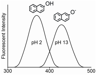
The most obvious thing to note is the large difference in the \(\lambda\)max value for the neutral 2-naphthol (355 nm) and the anionic 2-naphtholate ion (415 nm). The considerable difference between the two emission spectra occurs because the presence of more resonance forms leads to stabilization (i.e., lower energy) of the excited state. As shown in Figure \(\PageIndex{10}\), the 2-naphtholate species has multiple resonance forms involving the oxygen atom whereas the neutral 2-naphthol species only has a single resonance form. Therefore, the emission spectrum of the 2-naphtholate ion is red-shifted relative to that of the 2-naphthol species.

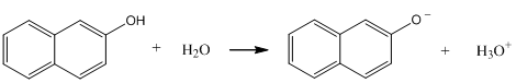
Consider the reaction shown below for the dissociation of 2-naphthol. This reaction may be either slow (slow exchange) or fast (fast exchange) on the time scale of fluorescence spectroscopy. Draw the series of spectra that would result for an initial concentration of 2-naphthol of 10-6 M if the pH was adjusted to 2, 8.5, 9.5, 10.5, and 13 and slow exchange occurred. Draw the spectra at the same pH when the exchange rate is fast.
If slow exchange occurs, an individual 2-naphthol or 2-naphtholate species stays in its protonated or deprotonated form during the entire excitation-emission process and emits its characteristic spectrum. Therefore, when both species are present in appreciable concentrations, two peaks occur in the spectrum for each of the individual species. On the left side of Figure \(\PageIndex{11}\), at pH 2, all of the species is in the neutral 2-naphthol form, whereas at pH 13 it is all in the anionic 2-naphtholate form. At pH 9.5, which equals the pKa value, there is a 50-50 mixture of the two and the peaks for both species are equal in intensity. At pH 8.5 and 10.5, one of the forms predominates. The intensity of each species is proportional to the concentration.
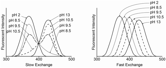
If fast exchange occurs, as seen on the right side of Figure \(\PageIndex{11}\), a particular species rapidly changes between its protonated and deprotonated form during the excitation and emission process. Now the emission is a weighted time average of the two forms. If the pH is such that more neutral 2-naphthol is present in solution, the maximum is closer to 355 nm (pH = 8.5). If the pH is such that more anionic 2-naphtholate is present in solution, the maximum is closer to 415 nm (pH = 10.5). At the pKa value (9.5), the peak appears in the middle of the two extremes.
What actually happens – is the exchange fast or slow? The observation is that the exchange of protons that occurs in the acid-base reaction is slow on the time scale of fluorescence spectroscopy. Remember that the lifetime of an excited state is about 10-8 second. This means that the exchange rate of protons among the species in solution is slower than 10-8 second and the fluorescence emission spectrum has peaks for both the 2-naphthol and 2-naphtholate species.
Devise a procedure that might allow you to determine the pKa of a weak acid such as 2-naphthol.
The pKa value of an acid is incorporated into an expression called the Henderson-Hasselbalch equation, which is shown below where HA represents the protonated form of any weak acid and A– is its conjugate base.
\[\mathrm{pH = pKa + \log \dfrac{[A^–]}{[HA]}} \nonumber \]
If a standard curve was prepared for 2-naphthol at a highly acidic pH and 2-naphtholate at a highly basic pH, the concentration of each species at different intermediate pH values when both are present could be determined. These concentrations, along with the known pH, can be substituted into the Henderson-Hasselbach equation to calculate pKa. As described earlier, this same process is used quite often in UV/VIS spectroscopy to determine the pKa of acids, so long as the acid and base forms of the conjugate pair have substantially different absorption spectra.
If you do this with the fluorescence spectra of 2-naphthol; however, you get a rather perplexing set of results in that slightly different pKa values are calculated at different pH values where appreciable amounts of the neutral and anionic form are present. This occurs because the pKa of excited state 2-naphthol is different from the pKa of the ground state. Since the fluorescence emission occurs from the excited state, this difference will influence the calculated pKa values. A more complicated set of calculations can be done to determine the excited state pKa values. UV/VIS spectroscopy is therefore often an easier way to measure the pKa of a species than fluorescence spectroscopy.
Because many compounds are weak acids or bases, and therefore the fluorescence spectra of the conjugate pairs might vary considerably, it is important to adjust the pH to insure all of either the protonated or deprotonated form.
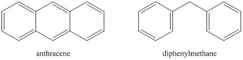
Which compound will have a higher quantum yield: anthracene or diphenylmethane?
Answering this question involves a consideration of the effect that collisions of the molecules will have in causing radiationless decay. Note that anthracene is quite a rigid molecule. Diphenylmethane is rather floppy because of the methylene bridge between the two phenyl rings. Hopefully it is reasonable to see that collisions of the floppy diphenylmethane are more likely to lead to radiationless decay than collisions of the rigid anthracene molecules. Another way to think of this is the consequences of a crash between a Greyhound bus (i.e., anthracene) and a car towing a boat (i.e., diphenylmethane). It might be reasonable to believe that under most circumstances, the car would suffer more damage in the collision.
Molecules that are suitable for analysis by fluorescence spectroscopy are therefore rigid species, often with conjugated \(\pi\) systems, that undergo less collisional deactivation. As such, fluorescence spectroscopy is a much more selective method than UV/VIS absorption spectroscopy. In many cases, a suitable fluorescent chromophore is first attached to the compound under study. For example, a fluorescent derivatization agent is commonly used to analyze amino acids that have been separated by high performance liquid chromatography. The advantage of performing such a derivatization step is because of the high sensitivity of fluorescence spectroscopy. Because of the high sensitivity of fluorescence spectroscopy, it makes it all the more important to control the variables described above as they will then have a more pronounced effect with the potential to cause errors in the measurement.