Part V: Ways to Draw Conclusions From Data

Investigation 26.

A z of 1.96 corresponds to a 95% confidence interval. Using Appendix 2, show that this is correct. What value of z corresponds to a 90% confidence inteval, and what value of z corresponds to a 99% confidence inteval? Report the 90%, the 95% and the 99% confidence intervals for the net weight of a single 1.69-oz bag of plain M&Ms drawn from a population for which μ is 48.98 g and σ is 1.433 g. For the data in Table 2, how many of the 30 samples have net weights that fall outside of the 90% confidence interval? Does this result make sense given your understanding of a confidence interval?

From the table in Appendix 2, we know that the area to the right of a z of 1.96 is 2.5% (a probability of 0.025) of the total area. Because the normal distribution is symmetrical, we know that the area to the left of a z of –1.96 also is 2.5% of the total area. The combined area of 5% is the percentage of samples excluded from the confidence interval; thus, the term ±zσ encompasses 95% of all samples, which is the meaning of a 95% confidence interval.

For a 90% confidence interval, we look for the value of z that corresponds to an area of 5%, which is a z of 1.645. For a 99% confidence interval, we look for the value of z that corresponds to an area of 0.5%, which is a z of 2.576. In both cases, the value of z is interpolated using the two neighboring values from the table. For example, from the table we see that z of 2.56 corresponds an area of 0.523% and a z of 2.58 corresponds to an area of 0.494%; to find the value z that corresponds to an area of 0.500% we set up the following equation

\[\dfrac{2.56 -z}{2.56 -2.58} =\dfrac{0.523 -0.500}{0.523 -0.494}\]

and solve for z, obtaining a result of 2.576.

The 90%, 95%, and 99% confidence intervals for a single 1.69-oz bag of plain M&Ms are

90% confidence interval: \(\textrm{48.98 g ± (1.645)(1.433 g) = 48.98 g ± 2.36 g}\)

95% confidence interval: \(\textrm{48.98 g ± (1.96)(1.433 g) = 48.98 g ± 2.81 g}\)

99% confidence interval: \(\textrm{48.98 g ± (2.576)(1.433 g) = 48.98 g ± 3.69 g}\)

For the data in Table 2, four of the samples have a net weight that falls outside of our 90% confidence interval, which extends from 46.62 g to 51.34 g; these samples are number 6 (46.405 g), number 29 (46.577 g), number 26 (51.682 g), and number 20 (51.730 g). With 30 samples and a 90% confidence interval, we expect, on average, to find that three samples have net weights that fall outside the confidence interval; finding four such samples is not an unreasonable outcome given that each sample represents just 3.3% of our pool of 30 samples.

Investigation 27.

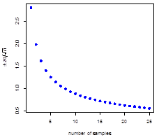
Suppose we draw four 1.69-oz bags of M&Ms from a population for which μ is 48.98 g and σ is 1.433 g. What are the 90%, the 95% and the 99% confidence intervals for the mean, \(\bar{x}\), of these samples? Prepare a plot that shows how n affects the width of the 95% confidence interval, expressed as \(±zσ/\sqrt{n}\), and discuss the significance of your plot. Suppose we wish to decrease the confidence interval by a factor of 3× solely by increasing the number of samples taken. If the original confidence interval is based on the mean of four samples, how many additional samples must we acquire?

The 90%, 95%, and 99% confidence intervals for the mean of four 1.69-oz bag of plain M&Ms are

90% confidence interval: \(\mathrm{48.98\: g ± (1.645)(1.433\: g) ⁄\sqrt{4} = 48.98\: g ± 1.18\: g}\)

95% confidence interval: \(\mathrm{48.98\: g ± (1.96)(1.433\: g) ⁄ \sqrt{4} = 48.98\: g ± 1.40\: g}\)

99% confidence interval: \(\mathrm{48.98\: g ± (12.576)(1.433\: g) ⁄ \sqrt{4} = 48.98\: g ± 1.85\: g}\)

Note that each confidence interval is half of that for the analysis of a single sample because the square root of the number of samples is two.

The figure below shows how the confidence interval changes as we increase the value of n from 1 to 25. The most important feature of this plot is to note how the rate at which the confidence interval’s width becomes smaller slows down as we increase the number of samples. For example, increasing the number of samples from one to four, decreases the confidence interval by a factor of 2× from ±2.81 to ±1.40. A further two-fold decrease in the confidence interval to ±0.70 requires 16 total samples, or an additional 12 samples.

To achieve a three-fold improvement in the width of the confidence interval—that is, a decrease in the confidence interval’s width by a factor of three—requires that we increase the number of samples from n₁ to n₂, where

\[\dfrac{\dfrac{zσ}{\sqrt{n_1}}}{\dfrac{zσ}{\sqrt{n_2}}}=\dfrac{\sqrt{n_2}} {\sqrt{n_1}}=3\]

Solving shows that the ratio n₂⁄n₁ is 3² or 9; thus, if the original confidence interval is based on four samples, then to achieve the desired smaller confidence interval we need a total of 9 × 4 = 36 samples, or an additional 32 samples.

Investigation 28.

Our data for 1.69-oz bags of plain M&Ms includes 30 measurements of the net weight. What are the 90%, the 95% and the 99% confidence intervals for the mean, \(\bar{x}\), of these samples? Using the 99% confidence interval as an example, explain the meaning of this confidence interval. Is the stated net weight of 1.69 oz a reasonable estimate of the true mean for the population of 1.69-oz bags of plain M&Ms?

The 90%, 95%, and 99% confidence intervals for the mean of 1.69-oz bag of plain M&Ms are

90% confidence interval: \(\mathrm{48.98\: g ± (1.699)(1.433\: g) ⁄\sqrt{30} = 48.98\: g ± 0.45\: g}\)

95% confidence interval: \(\mathrm{48.98\: g ± (2.045)(1.433\: g) ⁄ \sqrt{30} = 48.98\: g ± 0.54\: g}\)

99% confidence interval: \(\mathrm{48.98\: g ± (2.756)(1.433\: g) ⁄ \sqrt{30} = 48.98\: g ± 0.72\: g}\)

Using the 99% confidence interval as an example, and assuming that there are no errors in our measurements, there is a 99% probability that the confidence interval’s range of net weights—from a low of 48.26 g to a high of 49.70 g—includes the true mean for the population of all 1.69-oz bags of plain M&Ms; there is a 1% probability that population’s mean falls outside of this range. Given that the 99% confidence interval does not include the stated net weight of 1.69 oz (47.9 g), we can safely conclude that 1.69 oz is not a good estimate for the population’s mean net weight.

Investigation 29.

In 1996, Mars, the manufacturer of M&Ms, reported the following distribution for the colors of plain M&Ms: 30% brown, 20% red, 20% yellow, 10% blue, 10% green, and 10% orange. Pick any one color of M&Ms and, using the data in Table 2, calculate the percentage of that color in each of the 30 samples. Report the mean and the standard deviation for your color and use a t-test to determine whether your sample’s mean is consistent with the result reported by Mars. Gather results for the remaining five colors from other students and discuss your pooled results. Assuming that the distribution of colors reported by Mars is correct, what can you conclude about the manufacturing process.

For this problem the null hypothesis is \(H_0\textrm{: }\bar{x}=μ\) and the alternative hypothesis is \(H_A\textrm{: }\bar{x}≠μ\), where \(\bar{x}\) is the mean of the 30 samples for the color of interest and μ is the mean reported by Mars for the color of interest. The following table summarizes the results of the t-test, by color

color	\(\bar{x}\) (%)	s (%)	μ (%)	t	reject H0 at
brown	25.81	5.004	30	4.581	\(α\) < 0.01
red	17.64	6.600	20	1.962	0.05 < \(α\) <0.10
yellow	25.52	7.594	20	3.984	\(α\) < 0.01
blue	11.75	6.667	10	1.440	\(α\) > 0.10
green	6.52	4.743	10	4.018	\(α\) < 0.01
orange	12.75	4.983	10	3.024	\(α\) < 0.01

where s is the standard deviation for the 30 samples, t is the calculated experimental value of t based on \(\bar{x}\), s, and μ, and the last column defines the value of \(α\) for which we can reject the null hypothesis and accept the alternative hypothesis.

With the exception of the color blue, we have good evidence that the distribution of colors for these 30 samples is not in agreement with the manufacturer’s stated distribution. For brown, yellow, green, and orange, the 99% confidence interval does not include μ; for red, the 90% confidence interval does not include μ. These results are not particularly suprising. Although the distribution of colors in a production batch presumably matches the percentages provided by Mars, the mixing of the M&Ms at the level at which individual bags are filled likely is far from homogeneous.

In a response to a query regarding the proportions of colors in bags of M&Ms, the manufacturer noted that “[e]ach large production batch is blended to [this] ratio and mixed thoroughly. However, since the individual packages are filled by weight on high-speed equipment, and not by count, it is possible to have an unusual color distribution.” The full response can be seen here. It seems more likely that the color distribution is a function of sampling uncertainty associated with the population’s homogeneity at the level of sampling.