7.4: Titrimetic Methods of Analysis

7.4.1. “Classical” Redox Titration

A “classical” redox titration is one in which a titrant of a known concentration is prepared and standardized versus some appropriate primary standard. Then an accurate volume of an analyte solution with an unknown concentration is measured out. To be suitable for a titration, the analyte and titrant must undergo a rapid redox reaction that has a very large equilibrium constant so that formation of products is highly favored. The titrant is added from a burette and the volume needed to reach the endpoint is determined. The endpoint is identified through the use of an appropriate color-changing indicator. Besides an obvious color change, the criteria for selection of a suitable indicator is that it undergoes a redox reaction with the titrant that is less favored (has a lower equilibrium constant) than that of the analyte so that it only reacts after all of the analyte has reacted away. If the reaction between the titrant (TITR) and analyte (AN) is one-to-one, the following equation can be used to calculate the concentration (C) of the analyte.

\[\mathrm{C_{TITR} \times V_{TITR} = C_{AN} \times V_{AN}}\]

If the titrant and analyte react in something other than a one-to-one equivalency, then the above equation needs to be modified to reflect the proper stoichiometry.

7.4.2. Coulometric Titration (Controlled Current Coulometry)

A coulometric titration is an interesting variation on a classical redox titration. Consider the reaction below in which Fe²⁺ is the analyte and Ce⁴⁺ is the titrant. An examination of the two standard potentials for the two half reactions confirms that in this pair cerium will proceed as the reduction and iron as the oxidation.

\[\ce{Fe^2+(aq) + Ce^4+(aq) <=> Fe^3+(aq) + Ce^3+(aq)}\]

\[\ce{Ce^{4+}(aq) + e^- <=> Ce^{3+}(aq)} \mathrm{\hspace{40px} E^o = 1.61\: V}\]

\[\ce{Fe^{3+}(aq) + e^- <=> Fe^{2+}(aq)} \mathrm{\hspace{40px} E^o = 0.77\: V}\]

Rather than performing the titration by adding the Ce⁴⁺ from a burette, an excess of Ce³⁺ is added to an accurately measured volume of the unknown analyte solution. A constant electrochemical potential suitable to convert Ce³⁺ to Ce⁴⁺ is applied to the solution. As Ce⁴⁺ is produced, it immediately reacts with Fe²⁺ and is converted back to Ce³⁺. The result is that the concentration of Ce³⁺ is constant. A plot of the current measured by the generation of Ce⁴⁺ versus time would look like that in Figure 12.

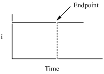
Figure 12. Plot of the current versus time in a coulometric titration.

There is more than one way to determine the endpoint of a coulometric titration. One is to add an indicator that reacts only when all the analyte is used up. In this case, you would measure the time until the color change and integrate the current versus time plot to determine the number of electrons and moles of analyte in the sample. Another possibility is that after the equivalence point, the “titrant” that is electrochemically generated no longer reacts away and there are other ways to measure that both members of the redox couple (Ce³⁺ and Ce⁴⁺ in the example above) are present.

What are some advantages of using a coulometric titration?

There are a number of advantages of a coulometric titration when compared to a classical redox titration.

• A coulometric titration has no burette.
• There is no need to standardize the titrant in a coulometric titration.All one has to do is add sufficient amounts of the titrant to the analyte solution (remember, we don’t actually add the titrant but add the appropriate species that will be converted into the titrant). Faraday’s constant is essentially the standard as it relates charge to the number of electrons and we know Faraday’s constant to a high degree of precision.
• Since we can accurately and precisely measure current and time, coulometric titrations are highly accurate and precise.
• Coulometric titrations are much more sensitive and can often measure lower concentrations than conventional titrations.
• Finally, because the titrant immediately reacts with the analyte after it is produced, it is possible to use an unstable titrant in a coulometric titration.Note that the species added to the solution that is converted into the titrant must be stable.

7.4.3. Amperometric Titration

An amperometric titration is done analogously to a classical titration in which a known volume of an analyte is measured out and a standardized titrant is added using a burette. The difference is that instead of using a color-changing indicator to determine the end point, the ability of the solution to generate a current is measured. It should be pointed out that you do not generate a large amount of current in an amperometric titration so the current generation does not deplete the solution of significant levels of the chemical species. Instead, you merely measure whether and how much current is produced at any given point during the titration.

\[\mathrm{Analyte + Titrant = Products}\]

A stipulation for monitoring a particular titration reaction amperometrically is that the products can never generate a current at the potential being applied to the system. What is also necessary is that the analyte and/or titrant are able to generate a current. This means that there are the three possible scenarios to consider for an amperometric titration.

Example \(\PageIndex{1}\):

Draw the plot of current (y-axis) versus ml of titrant (x-axis) if only the analyte generates a current.

Solution

In this case, at the beginning before any titrant is added there is a high concentration of analyte and therefore the current would be high. As titrant is added, it reduces the concentration of analyte leading to the formation of products and the current would drop. Since every similar increment of titrant reacts with the same amount of analyte, the current should decay in a linear manner and go to zero at the endpoint. The result is the plot seen in Figure 13.

Figure 13. Plot of current versus ml of titrant in an amperometric titration when only the analyte produces a current.

Example \(\PageIndex{2}\):

Draw the plot of current (y-axis) versus ml of titrant (x-axis) if only the titrant generates a current.

Solution

In this case, there is no current at the beginning because the analyte does not generate one. As small amounts of titrant are added, all of the titrant reacts with the analyte to form products so there is still no measureable current. In fact, up until the equivalence point, any added titrant reacts away. Only after the equivalence point and all of the analyte is used up is there extra unreacted titrant in the solution that produces a current. The result is the plot seen in Figure 14.

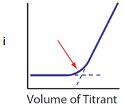
Figure 14. Plot of current versis ml of titrant in an amperometric titration when only the titrant produces a current.

Example \(\PageIndex{3}\):

Draw the plot of current (y-axis) versus ml of titrant (x-axis) if both the analyte and titrant generate a current.

Solution

The plot in this case is the combination of those in Figures 13 and 14. Prior to the equivalence point, there is analyte and a current is observed but diminishes as more titrant is added. After the equivalence point the concentration of unreacted titrant goes up so the current gets larger. The only point where there is no species in solution capable of generating a current is at the equivalence point. The result is the plot seen in Figure 15.

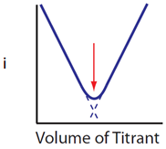
Figure 15. Plot of current versis ml of titrant in an amperometric titration when both the analyte and titrant produce a current.

7.4.4. Potentiometric Titration

The final titrimetric method we will examine is known as a potentiometric titration. This is similar to a classical titration as titrant is added from a burette. Instead of determining the endpoint using a color-changing indicator, a junction potential is continuously monitored during the titration. An example of a potentiometric titration that you are likely familiar with is a pH titration. In this case, a pH electrode is placed in the solution and the pH (determined by a membrane potential at the external glass membrane as described earlier in this unit) is measured continuously as titrant is added. The pH is plotted versus the ml of titrant added and there is a characteristic “break” or sharp rise in the plot that occurs at the equivalence point as seen in Figure 16. The plot has an inflection point that occurs at the equivalence point, although it is easier to identify the location of the inflection point by taking either the first or second derivative of the plot shown in Figure 16.

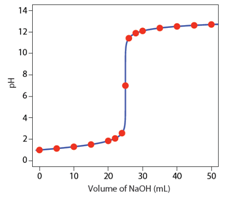
Figure 16. Plot of pH of a strong acid versus ml NaOH in a pH titration. (Figure from Analytical Chemistry 2.0, David Harvey, community.asdlib.org/activele...line-textbook/).

It is also possible to measure the progress of other redox reactions potentiometrically. For example, we could monitor the progress of the titration of a solution of Fe²⁺ using Ce⁴⁺ as the titrant. The products of the reaction are Fe³⁺ and Ce³⁺.

\[\mathrm{Fe^{2+}(aq) + Ce^{4+}(aq) = Fe^{3+}(aq) + Ce^{3+}(aq)}\]

The two relevant half reactions are shown below and indicate that the cerium reaction is the cathode and iron reaction is the anode.

\[\mathrm{Ce^{4+}(aq) + e^- = Ce^{3+}(aq) \hspace{40px} E^o = 1.61\: V}\]

\[\mathrm{Fe^{3+}(aq) + e^- = Fe^{2+}(aq) \hspace{40px} E^o = 0.77\: V}\]

Note that the E^o for the complete reaction is 0.84 V. Using the equation on p. 10 that relates E^o to K, the equilibrium constant for the reaction is greater than 10¹⁴. As with other electrochemical devices, a reference and working electrode is needed to perform the measurement. In this case, a platinum working electrode could be used. Let’s consider the following example to examine what will happen during the course of the titration and how one goes about calculating the potential during the titration.

Example \(\PageIndex{4}\):

20 ml of an 0.10 M solution of Fe²⁺ is titrated with 0.10 M Ce⁴⁺. Calculate the potential that would be measured when 5 ml, 10 ml, 20 ml, 30 ml and 40 ml of titrant have been added.

Solution

The following steps will allow us to work through the calculation of the junction potentials.

Write an expression for the total electrochemical potential of the titration reaction (this is the Nernst equation for the complete reaction).

\[\mathrm{E_{TOTAL}= E_{TOTAL}^0- \dfrac{0.059}{1} \log \dfrac{[Fe^{3+} ][Ce^{3+}]}{[Fe^{2+} ][Ce^{4+}]}}\]

Note, the reaction has one electron transferred between the cerium and iron so n = 1.

What is the total electrochemical potential of the titration reaction at any point during a titration? Think carefully about this because your first intuition may not be correct.

One of the criteria for any reaction to be useful in a titration is that the system must rapidly achieve equilibrium. What that means is that the titration above is always at equilibrium. In other words, when a drop of the cerium titrant is added, it immediately reacts with the iron and the system achieves equilibrium. Once past the equivalence point, there is some continuing distribution of species that occurs to establish equilibrium after each increment of titrant is added, but the system is always at equilibrium during all phases of the titration. That means that the total electrochemical potential of the reaction between Fe²⁺ and Ce⁴⁺ is zero at all points of the titration.

If we consider the other way we developed for determining the total electrochemical potential of a system.

\[\mathrm{E_{TOTAL} = E_{CATHODE} - E_{ANODE}}\]

Remember that when using this form of the equation, both the cathode and anode values are evaluated as reductions. Since we determined that E_Total = 0 at all steps for the titration reaction, the following relationship is valid throughout the titration:

\[\mathrm{E_{CATHODE} = E_{ANODE}}\]

However, there are two reactions to consider. One is the titration reaction and the other is the overall cell reaction. The overall cell reaction includes species in the reference electrode. Whereas the titration reaction goes to completion, the extent of the overall cell reaction is negligible because the voltmeter has high impedance that prevents current flow. The result is that the potential difference measured between the platinum and reference electrode during the titration is either the value E_CATHODE or E_ANODE developed above. Since these will both be equal, in theory either one of them could be used to calculate the potential at any point in the titration. However, there are advantages to using one of the half reactions over the other at certain points of the titration.

Which half reaction is easier to use to calculate the junction potential before the equivalence point? Which half reaction is easier to use after the equivalence point?

A way to consider this is to examine the amounts of the different species present at different points in the titration. The chart below shows the amounts of the different species in moles as the titration progresses.

Titrant (ml)	Fe^2+	Ce^4+	Fe^3+	Ce^3+
0	0.0020 m	0 m	0 m	0 m
5 ml	0.0015 m	0 m	0.0005 m	0.0005 m
10 ml	0.0010 m	0 m	0.0010 m	0.0010 m
20 ml	0 m	0 m	0.0020 m	0.0020 m
30 ml	0 m	0.0010 m	0.0020 m	0.0020 m
40 ml	0 m	0.0020 m	0.0020 m	0.0020 m

It is important to note that except for the first line when no titrant has been added, the concentrations listed as “0 m” are not actually zero. Because the equilibrium constant for the reaction has a finite value, the concentration of each species must be a finite value. However, the equilibrium constant for this reaction is large (>10¹⁴), so the redistribution or back reaction of species that occurs involves only a small amount. As an example, let’s consider the values at 5 ml.

5 ml Titrant	Fe^2+	Ce^4+	Fe^3+	Ce^3+
Initial	0.0015 m	0 m	0.0005 m	0.0005 m
Back reaction	0.0015 + X m	X m	0.0005 – X m	0.0005 – X m
Approximation	0.0015	X m	0.0005	0.0005 m

For the line labeled “back reaction”, a small amount (X) of the Fe³⁺ and Ce³⁺ are removed to generate some Ce⁴⁺ and Fe²⁺. However, the value of X is so small relative to 0.00050 and 0.0015 moles (again because K is so large) that it is insignificant and can be ignored. Therefore, the amounts shown in the line labeled “approximation” can be used for any calculations.

An important outcome that arises by examining the amounts in the chart above is that prior to the equivalence point (5 and 10 ml of titrant) there are appreciable amounts of both Fe²⁺ and Fe³⁺. That means it will be preferable to use the iron half reaction in calculating the junction potential before the equivalence point.

Also note that after the equivalence point (30 and 40 ml of titrant) there are appreciable amounts of both Ce³⁺ and Ce⁴⁺. That means it will be preferable to use the cerium half reaction in calculating the junction potential after the equivalence point.

We can now calculate the values before and after the equivalence point.

5 ml

\[\mathrm{E_{Fe}= E_{Fe}^0- \dfrac{0.059}{1} \log \dfrac{[Fe^{2+}]}{[Fe^{3+}]}}\]

\[\mathrm{E_{Fe}=0.77- \dfrac{0.059}{1} \log \dfrac{[0.0015\: m]}{[0.0005\: m]} =0.74\: V}\]

There is one other important thing to note in this calculation. Because we have a ratio of [Fe²⁺] to [Fe³⁺] in the log term, the volumes associated with the two concentrations cancel each other out. So using the number of moles of the two species when there are appreciable amounts of both gives the same value as using the concentration.

10 ml

\[\mathrm{E_{Fe}= E_{Fe}^0- \dfrac{0.059}{1} \log \dfrac{[Fe^{2+}]}{[Fe^{3+}]}}\]

\[\mathrm{E_{Fe}=0.77- \dfrac{0.059}{1} \log \dfrac{[0.0010\: m]}{[0.0010\: m]} =0.77\: V}\]

Note that in this case, with the concentrations of Fe²⁺ and Fe³⁺ being equal, the log of 1 is zero and the potential is equal to E^o_Fe.

30 ml

\[\mathrm{E_{Ce}= E_{Ce}^0- \dfrac{0.059}{1} \log \dfrac{[Ce^{3+}]}{[Ce^{4+}]}}\]

\[\mathrm{E_{Fe}=1.61- \dfrac{0.059}{1} \log \dfrac{[0.0010\: m]}{[0.0020\: m]} =1.59\: V}\]

40 ml

\[\mathrm{E_{Ce}= E_{Ce}^0- \dfrac{0.059}{1}\log\dfrac{[Ce^{3+}]}{[Ce^{4+}]}}\]

\[\mathrm{E_{Fe}=1.61- \dfrac{0.059}{1} \log \dfrac{[0.0020\: m]}{[0.0020\: m]} =1.61\: V}\]

Note that in this case, with the concentrations of Ce³⁺ and Ce⁴⁺ being equal, the log of 1 is zero and the potential is equal to E^o_Ce.

The only item remaining potential to be calculated is at the equivalence point where we cannot easily use either of the two half reactions to calculate the potential. Using the two half reactions and knowledge of the stoichiometric equivalence of the different species at the equivalence point, It is possible to derive the following generalizable equation for the potential that will be measured at the equivalence point. A and B refer to the two half reactions and n_A and n_B are the number of electrons in each of the half reactions, respectively.

\[\mathrm{E_{Eq.Pt.}= \dfrac{(n_A E_A^0+ n_B E_B^0)}{(n_A+ n_B)}}\]

For the reaction in our problem, n_A and n_B are both 1 so the result is that the equivalence point potential is the average of the two E^o values.

\[\mathrm{E_{Eq.Pt.}= \dfrac{(0.77+ 1.61)}{(2)}=1.19\: V}\]

The chart below summarizes the potential measured at different points in the titration.

Titrant (ml)	Fe^2+	Ce^4+	Fe^3+	Ce^3+	Potential
5 ml	0.0015 m	0 m	0.0005 m	0.0005 m	0.74 V
10 ml	0.0010 m	0 m	0.0010 m	0.0010 m	0.77 V (E^oFe)
20 ml	0 m	0 m	0.0020 m	0.0020 m	1.19 V
30 ml	0 m	0.0010 m	0.0020 m	0.0020 m	1.59 V
40 ml	0 m	0.0020 m	0.0020 m	0.0020 m	1.61 V (E^oCe)

A plot of the potential (y-axis) versus the ml of titrant (x-axis) is shown in Figure 17.

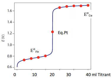
Figure 17. Plot of potential versus ml titrant for the potentiometric titration of Fe²⁺ with Ce⁴⁺. (Figure from Analytical Chemistry 2.0, David Harvey, community.asdlib.org/activele...line-textbook/).

The break in potential that occurs at the equivalence point is apparent in this plot. Note how the general form of this plot is similar to what is observed in a pH titration. This is not surprising since a pH titration is also a potentiometric titration.

One last thing worth examine is the equivalence point potential for a redox reaction where the number of electrons is different in each of the half reactions. For example, suppose Sn²⁺ was titrated with Ce⁴⁺. The two relevant half reactions are shown below.

\[\mathrm{Ce^{4+}(aq) + e^- = Ce^{3+}(aq) \hspace{40px} E^o = 1.61\: V}\]

\[\mathrm{Sn^{4+}(aq) + 2e^- = Sn^{2+}(aq) \hspace{40px} E^o = 0.154\: V}\]

In this case, the balanced reaction needs two equivalents of Ce⁴⁺ for each Sn²⁺ to balance out the electrons being transferred.

\[\mathrm{Sn^{2+}(aq) + 2Ce^{4+}(aq) = Sn^{4+}(aq) + 2Ce^{3+}(aq)}\]

The equivalence point potential is calculated as follows:

\[\mathrm{E_{Eq.Pt.}= \dfrac{(n_A E_A^0+ n_B E_B^0)}{(n_A+ n_B)}}\]

\[\mathrm{E_{Eq.Pt.}= \dfrac{(E_{Ce}^0+ 2E_{Sn}^0)}{(1+2)}}\]

\[\mathrm{E_{Eq.Pt.}= \dfrac{(1.61+ 2(0.154))}{(3)}=0.639\: V}\]

The plot of potential versus ml titrant that would be obtained for this titration is shown in Figure 18.

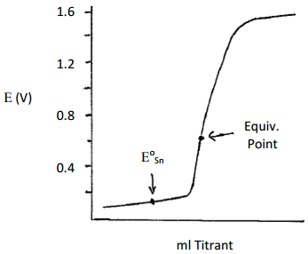
Figure 18. Plot of potential versus ml titrant for the potentiometric titration of Sn²⁺ with Ce⁴⁺.

It is important to note that the equivalence point in Figure 18 is not symmetrically placed between the two potential plateaus surrounding the E^o value of tin and E^o value of cerium as it was in the reaction of cerium and iron we examined earlier. Instead, the equivalence point potential is weighted toward the E^o value of tin because the tin half reaction requires two electrons whereas the cerium half reaction only requires one.