Part V. Optimizing the Solvent-to-Solid Ratio and the Extraction Time

Investigation 19

When optimizing the choice of solvent, temperature, and microwave power, we used absorbance values taken directly from the HPLC analysis (see Figures 3–8) without first converting them into extraction yields reported in mg analyte/g sample. Why is it possible to use absorbance values for the optimizations in Part IV? Can you use absorbance values when optimizing the solvent-to-solid ratio or the extraction time? Why or why not? Using the optimum conditions from Figure 8 and your results from Investigation 7, report the extraction yield for each analyte as mg analyte/g sample.

It helps to begin by considering how to convert an analyte’s peak height in mAU to the analyte’s extraction yield in mg/g. We know from Investigations 6 and 7 that Beer’s law is A = kC, where A is the analyte’s absorbance, C is the analyte’s concentration in the extracting solvent (in μg/mL), and k is an analyte-specific calibration constant (with units of mAU•mL/μg); thus

\[C= \dfrac{A}{k}\nonumber\]

To convert C to the analyte’s extraction yield, EY, we account for the volume of solvent, V, and the mass of sample, m

\[EY\left(\mathrm{\dfrac{mg}{g}}\right)=\dfrac{C\left(\mathrm{\dfrac{μg}{mL}}\right)×V\mathrm{(mL)}}{m\: \mathrm{(g)}}×\mathrm{\dfrac{1\: mg}{1000\: μg}}=\dfrac{A \mathrm{(mAU)}×V\mathrm{(mL)}}{k\mathrm{\left(\dfrac{mAU•mL}{μg}\right)}× m\: \mathrm{(g)}}×\mathrm{\dfrac{1\: mg}{1000\: μg}}\nonumber\]

When optimizing the choice of solvent, extraction temperature, and microwave power, we maintained a constant solvent-to-solid ratio, using 60.0 mL of solvent and a 3.00-g sample for each experiment. Because V, k, and m, are constants, the analyte’s absorbance and its extraction yield are directly proportional: if the absorbance doubles, we know the extraction yield also doubles. This is why we can use absorbance values when optimizing the choice of solvent, the extraction temperature, and the microwave power.

To optimize the solvent-to-solid ratio we must change the solvent’s volume and/or the sample’s mass, which means we no longer can assume that an increase in the analyte’s absorbance evinces a proportionate increase in the analyte’s extraction yield; instead, we must calculate the analyte’s extraction yield from its absorbance. The following table summarizes the extraction yields for the optimum extraction conditions in Figure 8.

analyte	absorbance (mAU)	k (mAU•mL/μg)	EY (mg/g)
danshensu	064.4	1.605	0.802
rosmarinic acid	098.9	0.878	2.253
lithospermic acid	062.2	0.536	2.320
salvianolic acid A	042.3	1.585	0.534
dihydrotanshinone	065.8	2.841	0.463
cryptotanshinone	084.4	1.882	0.897
tanshinone I	104.4	1.599	1.306
tanshinone IIA	201.9	1.467	2.752

Investigation 20

We can divide the points in a central-composite design into three groups: a set of points that allow us to explore the effect on the extraction yield of extraction time only; a set of points that allow us to explore the effect on the extraction yield of the solvent-to-solid ratio only; and a set of points that allow us to explore the effect on the extraction yield of the interaction between extraction time and the solvent-to-solid ratio. Explain how each of these is accomplished in this experimental design.

For the points (2.18, 25.0), (5.00, 25.0), and (7.82, 25.0) we are changing the extraction time while maintaining a constant solvent-to-solid ratio; these points allow us to explore the effect of extraction time only. For the points (5.00, 10.9), (5.00, 25.0), and (5.00, 39.1) we are changing the solvent-to-solid ratio while maintaining a constant extraction time; these points allow us to explore the effect of the solvent-to-solid ratio only. Finally, for the points (3.00, 15.0), (7.00, 15.0), (3.00, 35.0), and (7.00, 35.0) we vary both the extraction time and the solvent-to-solid ratio; these points allow us to explore possible interactions between these factors.

Note: In Table 1 of the original paper, the extraction time’s lower limit and upper limit are reported as 2.00 min and 8.00 min, respectively, instead of 2.18 min and 7.82 min, as used in this case study. The original paper also reports the lower limit and the upper limit for the solvent-to-solid ratio as 10.0 mL/g and 40.0 mL/g, respectively, instead of 10.9 mL/g and 39.1 mL/g, as used in this case study. This is the result of an inconsistency in the original paper between the reported actual factor levels and the reported coded factor levels used for building a regression model. If, as the paper indicates, the experimental design’s axial points are ±1.41, then the reported factor levels of 2.00 min, 8.00 min, 10.0 mL/g, and 40.0 mL/g are in error and should be listed as 2.18 min, 7.82 min, 10.9 mL/g, and 39.1 mL/g, respectively. On the other hand, if the reported factor levels of 2.00 min, 8.00 min, 10.0 mL/g, and 40.0 mL/g are correct, then the reported coded factor levels of ±1.41 are in error and should be listed as ±1.50. For the purpose of this case study, we assume the axial point’s coded factor levels are ±1.41 and that 2.18 min, 7.82 min, 10.9 mL/g, and 39.1 mL/g are the actual factor levels for these points. Fortunately, the effect on the regression results of this inconsistency is not important within the context of this case study. See the comments accompanying Investigation 23 for additional details.

Investigation 21

Identify the five trials at the center of central-composite design and, for these trials, calculate the extraction yield’s mean, standard deviation, relative standard deviation, variance, and 95% confidence interval about the mean. What is the statistical meaning for each of these values? Transfer to Figure 9 the extraction yield for each experiment, using the mean extraction yield for the design’s center point. What conclusions can you reach regarding the effect on danshensu’s extraction yield of extraction time and solvent-to-solid ratio? Estimate the optimum conditions for maximizing danshensu’s extraction yield and explain your reasoning?

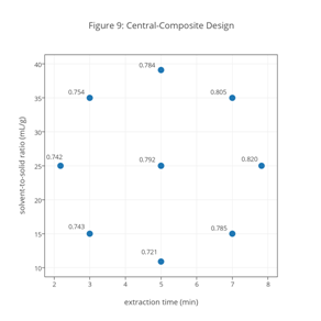
The center of the central-composite design is an extraction time of 5.00 min and a solvent-to-solid ratio of 25.0 mL/g. The extraction yields for these five trials are 0.790, 0.813, 0.785, 0.801, and 0.773. The mean, which is 0.792 mg/g, is the average value for the five trials and is our best estimate of danshensu’s true extraction yield, μ, in the absence of systematic errors in the analysis. The standard deviation of 0.0153 is one measure of the dispersion about the mean for these five trials. Two other measures of dispersion are the relative standard deviation, the ratio of the standard deviation to the mean, which is 1.93% in this case, and the variance, which is the square of the standard deviation, or 2.34×10^–4 in this case. The standard deviation, relative standard deviation, and variance each provide a measure of the uncertainty in our results resulting from random error in the extraction and analysis. The 95% confidence interval combines the mean and the standard deviation to estimate danshensu’s true extraction yield when using an extraction time of 5.00 min and a solvent-to-solid ratio of 25 mL/g. Its value is given by

\[μ=\bar{X} ±\dfrac{ts}{\sqrt{n}}\nonumber\]

where \(\bar{X}\) is the mean, s is the standard deviation, n is the number of trials, and t is a value that depends on the confidence level and the degrees of freedom, which is n – 1. The value of t for a 95% confidence interval and n = 5 (four degrees of freedom) is 2.776; the 95% confidence interval is

\[0792±\dfrac{(2.776×0.0152)}{\sqrt{5}}=0.792±0.019\nonumber\]

This confidence interval is important because it helps us evaluate whether a change in a factor’s level affects the extraction yield. Consider, for example, the extraction yields of 0.742, 0.792, and 0.820 for the three points that include a change in extraction time only: (2.18, 25.0), (5.00, 25.0), and (7.82, 25.0). If extraction time does not affect the extraction yield, then we expect the extraction yields at (2.18, 25.0) and at (7.82, 25.0) to fall within the 95% confidence interval around the mean value at (5.00, 25.0). The actual yields do not fall with this range, suggesting that extraction time does affect danshensu’s extraction yield, with longer extraction times favoring greater extraction yields.

A similar analysis of the data for the points (5.00, 10.9), (5.00, 25.0), and (5.00, 39.1) suggests that the solvent-to-solid ratio significantly affects the extraction yields, with solvent-to-solid ratios less than 25.0 mL/g resulting in a decrease in the extraction yield. Finally, the data for the points (3.00, 15.0), (7.00, 15.0), (3.00, 35.0), and (7.00, 35.0) suggests that the interaction between the extraction time and the solvent-to-solid ratio is not significant. For example the effect on the extraction yield of a change in extraction time when the solvent-to-solid ratio is 35.0 is

\[0.805 - 0.754 = 0.051\nonumber\]

and the effect on the extraction yield of a change in extraction time when the solvent-to-solid ratio is 15.0 is

\[0.785 - 0743 = 0.042\nonumber\]

The difference between these values

\[0.051 - 0.042 = 0.009\nonumber\]

is smaller than the 95% confidence interval, suggesting that the difference is not significant and that these are independent, not dependent factors (see Investigation 10).

Based on Figure 9, the optimum condition for extracting danshensu is an extraction time of 7.80 min and a solvent-to-solid ratio of 25.0 mL/g as this yields the greatest extraction yield.

Investigation 22

What does it mean to describe a model as empirical instead of theoretical? What are the advantages and the disadvantages of using an empirical model? What is the significance for this empirical model of the coefficients β₀, β_a, β_b, β_aa, β_bb, and β_ab? How does an empirical model that includes the coefficients β_aa and β_bb differ from a model that does not include these coefficients?

For an empirical model there is no established mathematical relationship between the response and the factors affecting the response. To fit an empirical model to data, we search for a mathematical expression that reasonably fits the data, which means an empirical model is not independent of the data used to build the model. A theoretical model, as its name suggests, is derived from a theoretical understanding of the relationship between the response and the factors affecting the response; as such, a theoretical model is independent of the data we may wish to model. Although a theoretical model can emerge from the understanding engendered by an empirical model, it still must be explained in terms of existing theory. Boyle’s law (PV = constant) is an example of an empirical model that emerged from the careful study of the relationship between a gas’s pressure and its volume. The derivation of Boyle’s law from the kinetic theory of gases transformed Boyle’s law from an empirical model to a theoretical model.

The advantage of an empirical model is that it allows us to model a response, such as an extraction yield, when there is no existing theoretical model that explains the relationship between the response and its factors. The disadvantage of an empirical model is that its utility is limited to the range of factor levels studied. For example, we might use a straight-line

\[y=β_0+β_x x\nonumber\]

to successfully model a response, y, over a limited range of levels for a factor, x, even though the relationship between y and x over a wider range of levels is much more complex. If we use the model to predict values of y for values of x within the range modeled, a process we call interpolation, then we are confident in our results; attempting to predict values of y for values of x outside of the range modeled, a process we call extrapolation, is likely to introduce substantial errors into our analysis.

For the empirical model in this exercise the coefficient β₀ is the intercept, the coefficients β_a and β_aa provide the first-order and second-order effects on the response of extraction time, the coefficients β_b and β_bb provide the first-order and second-order effects on the response of the solvent-to-solid ratio, and β_ab provides the interaction between the extraction time and the solvent-to-solid ratio. A model that includes the coefficients β_aa and β_bb allows for curvature in the response surface; a response surface without these coefficients is a flat plane.

Investigation 23

What does it mean to say that the regression analysis is significant at p = 0.0057? Do the results of this regression analysis, as expressed in the model’s coefficients, agree with your results from Investigation 21? Why or why not? What is the meaning of the intercept in this model and how does it affect your understanding of the empirical model’s validity? Use the full regression model to calculate danshensu’s predicted extraction yields for the central-composite design in Table 2. Organize your results in a table with columns for the factor levels, the experimental extraction yields, and the predicted extraction yields. Add a column showing the difference between the experimental extraction yields and predicted extraction yields. Calculate the mean, standard deviation, and the 95% confidence interval for these difference values and comment on your results.

In a linear regression analysis, we want to determine if a factor’s levels affect the response or if the response is independent of the factor’s levels. For each experiment used to build the model, we consider three possible responses: the measured response, \(y_i\), the response predicted by the model, \(\hat{y}_i\), and the average response over all experiments, \(\bar{y}\), which is our best estimate of the response if it is independent of the factors. If the total difference between the experimental responses and the average response, \(∑(y_i-\bar{y})^2\), is signficantly greater than the total difference between the experimental responses and the predicted responses, \(∑(y_i-\hat{y}_i )^2\), then we have evidence that random errors in our measurements cannot explain the differences in experimental responses; that is, we have evidence that the response is dependent on the factors. A p value of 0.0057 means there is but a 0.57% probability that random error can account for the differences in the extraction yields reported in Table 2. Note that a regression analysis can not prove that a model is correct, but it does provide confidence that the model does a better job of explaining the experimental data than does random error.

In Investigation 21 we concluded that an increase in extraction time increases the extraction yield and that a decrease in the solvent-to-solid ratio results decreases the extraction yield; both of these conclusions are consistent with the positive values for β_a and β_b, and consistent with their p values. We also concluded that there was no evidence for a significant interaction between the extraction time and the solvent-to-solid ratio, which is consistent with β_ab not having a p value less than 0.05 (it actually is >0.7). Interestingly, the model suggests that the solvent-to-solid ratio has a significant second-order effect on the response as the p value for β_bb is less than 0.05, a conclusion we did not draw in Investigation 21.

The intercept for this model gives the extraction yield for an extraction time of 0 min and a solvent-to-solid ratio of 0 mL/g. That the intercept is not 0 mg/g and that it is highly significant seems troubling; after all, how we can extract the analyte if we do not use solvent and if we do not carry out the extraction! Here is where we need to recall that we are using an empirical model to explain the relationship between the factors and the response. As noted in Investigation 22, we cannot extrapolate an empirical model outside the range of the factor levels used to build the model. In this case, we cannot safely predict extraction yields for extraction times less than 2.18 min or for solvent-to-solid ratios of less than 10.9 mL/g.

The following table compares the experimental extraction yields from Table 2 with the extraction yields predicted using our model.

extraction time (min)	solvent-to-solid ratio (mL/g)	experimental extraction yield (mg/g)	predicted extraction yield (mg/g)	difference (mg/g)
5.00	10.9	0.721	0.741	–0.020
5.00	25.0	0.790	0.792	00.002
3.00	15.0	0.743	0.734	­–0.009
2.18	25.0	0.742	0.747	00.005
3.00	35.0	0.754	0.756	00.002
5.00	25.0	0.813	0.792	–0.021
7.00	15.0	0.785	0.780	–0.005
5.00	25.0	0.785	0.792	00.007
5.00	39.1	0.784	0.777	–0.007
7.00	35.0	0.805	0.810	00.005
5.00	25.0	0.801	0.792	–0.009
5.00	25.0	0.773	0.792	00.019
7.82	25.0	0.820	0.817	–0.003

The mean difference between the predicted extraction yields and the experimental extraction yield is –4.6×10^–4 with a standard deviation of 0.011 and a 95% confidence interval (t = 2.179 for 12 degrees of freedom) of ±0.0069. The mean difference is small, as we expect if the model explains our data, and there is no evidence that it deviates significantly from 0. For three trials—highlighted above in bold—the differences between the predicted extraction yields and the experimental extraction yields are more than twice the 95% confidence interval; nevertheless, the agreement between the experimental and the predicted extraction yields is encouraging.

Note: The regression models in the original paper are reported using coded factor levels, which normalize each factor’s level so that each factor has the same scale. The equation for the regression model provided in this exercise translates back into the actual factor levels the coded regression model reported in the original paper. A regression analysis of the data in Table 1 of the original paper yields results that are slightly different than those reported in Table 2 of the original paper. This is not a result of uncertainty in the assignment of coded levels for the central-composite design’s axial points, as described in the notes accompanying Investigation 20. As shown here

coefficient	reported in paper using ±1.41	calculated using ±1.41	calculated using ±1.5
β0	00.7920	00.7920	00.7930
βa	00.0250	00.0254	00.0254
βb	00.0130	00.0150	00.0148
βaa	–0.0050	–0.0044	–0.0046
βbb	–0.0165	–0.0187	00.0173
βab	00.0020	00.0022	00.0022

a regression analysis of the extraction yields using coded factor levels of ±1.41 for the axial points and using coded factor levels of ±1.5 give coefficients (in coded form) that look similar to each other, but that are not the same as those reported in Table 2 of the original paper. A more likely explanation is that the reported extraction yields in Table 1 of the original paper are the average of three trials; although not stated, the regression results reported in the original paper presumably uses the full set of individual extraction yields instead of the average extraction yields, as is the case here.

Investigation 24

Does Figure 10 agree with your results from Investigations 21 and 23? Why or why not? Estimate the optimum conditions for maximizing danshensu’s extraction yield and explain your reasoning. How sensitive is the optimum extraction yield to a small change in extraction time? How sensitive is the optimum extraction yield to a small change in the solvent-to-solid ratio?

The shape of the response surface is consistent with our observations from earlier investigations. The contour lines show that the extraction yield increases for longer extraction times (as seen in both Investigations 21 and 23), and shows that the extraction yield decreases both for larger and for smaller solvent-to-solid ratios (as seen in Investigation 23). The contour lines are more spherical than elliptical, which is consistent with a model that does not have a significant interaction between its factors (as seen in Investigations 21 and 23).

In Investigation 21, we concluded that the optimum condition for extracting danshensu is an extraction time of 7.80 min and a solvent-to-solid ratio of 25.0 mL/g with an extraction yield of 0.817. Based on the response surface, the optimum condition for extracting danshensu is an extraction time of 7.80 min and a solvent-to-solid ratio of 35.0 mL/g with an extraction yield of 0.821; the difference in the extraction yields, however, is not significant and is consistent with the response surface’s broad contours at longer extraction times.

The relative sensitivity of a response to a change in a factor’s level is indicated by the steepness of the slope along the direction of that change (consider, for example, the closely spaced contour lines on a topographic map for a deep canyon compared to the widely spaced contour line for a gently sloping field). For danshensu, the optimum extraction yield is equally sensitive to a change in the extraction time and the solvent-to-solid ratio, although the sensitivity is small given that the optimum is on a broad hill with a shallow slope.

Investigation 25

Using Figures 11–15, determine the optimum extraction time and solvent-to-solid ratio for lithospermic acid, salvianolic acid A, cryptotanshinone, tanshinone I, and tanshinone IIA. How sensitive is the extraction of each analyte to a small change in the optimum extraction time and in the optimum solvent-to-solid ratio? Considering your responses here and to Investigation 24, are there combinations of extraction times and solvent-to-solid ratios that will optimize the extraction yield for all six of these analytes?

The following table summarizes the maximum extraction yields and the optimum extraction times and solvent-to-solid ratios from Figures 11–15, with the results for danshensu, from Investigation 24, included as well.

analyte	extraction time (min)	solvent-to-solid ratio (mL/g)	maximum extraction yield (mg/g)
danshensu	7.80	35.0	0.821
lithospermic acid	7.80	39.0	2.784
salvianolic acid A	7.80	39.0	0.624
cryptotanshinone	7.80	34.5	0.920
tanshinone I	7.80	31.5	1.353
tanshinone IIA	6.20	34.5	2.784

The optimum conditions for extracting cryptotanshinone, tanshinone I, and tanshinone IIA, which sit on plateaus or ridges with shallow slopes, are not particularly sensitive to small changes in the extraction time or the solvent-to-solid ratio. The optimum conditions for extracting lithospermic acid and salvianolic acid A are on more steeply rising slopes and, therefore, are more sensitive to a change in either the extraction time or the solvent-to-solid ratio.

For all six analytes, longer extraction times and larger solvent-to-solid ratios favor a greater extraction yield; however, as the table above shows, the optimum extraction yield for tanshinone IIA has a shorter extraction time than the other five analytes, and the optimum extraction yield for lithospermic acid and for salvianolic acid A favors a larger solvent-to-solid ratio. How to determine a single set of extraction conditions is the subject of Part VI.

Note: Figures 11–15 use the regression results reported in Table 2 of the original paper. The value of β_ab for tanshinone I is reported in Table 2 as 0.247 instead of its more likely value of 0.0247, which was used to generate Figure 14; unlike the corrected value, the reported value does not produce a response surface consistent with that shown in Figure 7b of the original paper. As noted in the case study, the regression models are not significant for rosmarinic acid and for dihydrotanshinone; the extraction yields of 2.317 mg/g for rosmarinic acid and 0.424 mg/g for dihydrotanshinone reported in the exercise are the average of the five replicate trials at the center of the central-composite design.