7.3: X-ray Crystallography
- Page ID
- 55906

An Introduction to X-ray Diffraction
History of X-ray Crystallography
The birth of X-ray crystallography is considered by many to be marked by the formulation of the law of constant angles by Nicolaus Steno in 1669 (Figure \(\PageIndex{1}\)).
Although Steno is well known for his numerous principles regarding all areas of life, this particular law dealing with geometric shapes and crystal lattices is familiar ground to all chemists. It simply states that the angles between corresponding faces on crystals are the same for all specimens of the same mineral. The significance of this for chemistry is that given this fact, crystalline solids will be easily identifiable once a database has been established. Much like solving a puzzle, crystal structures of heterogeneous compounds could be solved very methodically by comparison of chemical composition and their interactions.

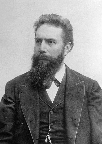
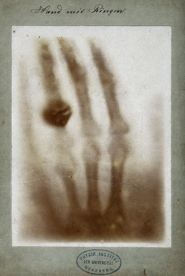
Although Steno was given credit for the notion of crystallography, the man that provided the tools necessary to bring crystallography into the scientific arena was Wilhelm Roentgen (Figure \(\PageIndex{2}\)), who in 1895 successfully pioneered a new form of photography, one that could allegedly penetrate through paper, wood, and human flesh; due to a lack of knowledge of the specific workings of this new discovery, the scientific community conveniently labeled the new particles X-rays. This event set off a chain reaction of experiments and studies, not all performed by physicists. Within one single month, medical doctors were using X-rays to pinpoint foreign objects such in the human body such as bullets and kidney stones (Figure \(\PageIndex{3}\)).
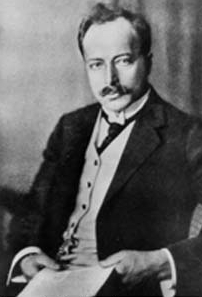
The credit for the actual discovery of X-ray diffraction goes to Max von Laue (Figure \(\PageIndex{4}\), to whom the Nobel Prize in physics in 1914 was awarded for the discovery of the diffraction of X-rays. Legend has it that the notion that eventually led to a Nobel prize was born in a garden in Munich, while von Laue was pondering the problem of passing waves of electromagnetic radiation through a specific crystalline arrangement of atoms. Because of the relatively large wavelength of visible light, von Laue was forced to turn his attention to another part of the electromagnetic spectrum, to where shorter wavelengths resided. Only a few decades earlier, Röentgen had publicly announced the discovery of X-rays, which supposedly had a wavelength shorter than that of visible light. Having this information, von Laue entrusted the task of performing the experimental work to two technicians, Walter Friedrich and Paul Knipping. The setup consisted of an X-ray source, which beamed radiation directly into a copper sulfate crystal housed in a lead box. Film was lined against the sides and back of the box, so as to capture the X-ray beam and its diffraction pattern. Development of the film showed a dark circle in the center of the film, surrounded by several extremely well defined circles, which had formed as a result of the diffraction of the X-ray beam by the ordered geometric arrangement of copper sulfate. Max von Laue then proceeded to work out the mathematical formulas involved in the observed diffraction pattern, for which he was awarded the Nobel Prize in physics in 1914.
Principles of X-Ray Diffraction (XRD)
The simplest definition of diffraction is the irregularities caused when waves encounter an object. Diffraction is a phenomenon that exists commonly in everyday activities, but is often disregarded and taken for granted. For example, when looking at the information side of a compact disc, a rainbow pattern will often appear when it catches light at a certain angle. This is caused by visible light striking the grooves of the disc, thus producing a rainbow effect (Figure \(\PageIndex{5}\)), as interpreted by the observers' eyes. Another example is the formation of seemingly concentric rings around an astronomical object of significant luminosity when observed through clouds. The particles that make up the clouds diffract light from the astronomical object around its edges, causing the illusion of rings of light around the source. It is easy to forget that diffraction is a phenomenon that applies to all forms of waves, not just electromagnetic radiation. Due to the large variety of possible types of diffractions, many terms have been coined to differentiate between specific types. The most prevalent type of diffraction to X-ray crystallography is known as Bragg diffraction, which is defined as the scattering of waves from a crystalline structure.

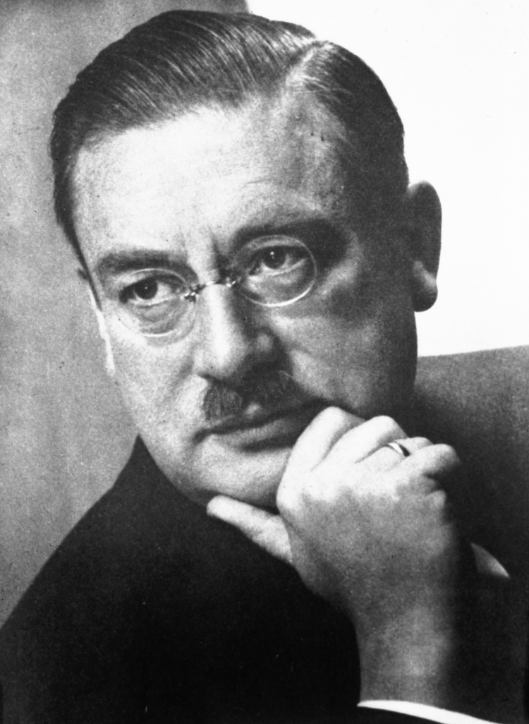
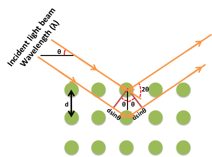
Formulated by William Lawrence Bragg (Figure \(\PageIndex{6}\)), the equation of Bragg's law relates wavelength to angle of incidence and lattice spacing, \ref{1}, where n is a numeric constant known as the order of the diffracted beam, λ is the wavelength of the beam, d denotes the distance between lattice planes, and θ represents the angle of the diffracted wave. The conditions given by this equation must be fulfilled if diffraction is to occur.
\[ n\lambda \ =\ 2d\ sin(\theta ) \label{1} \]
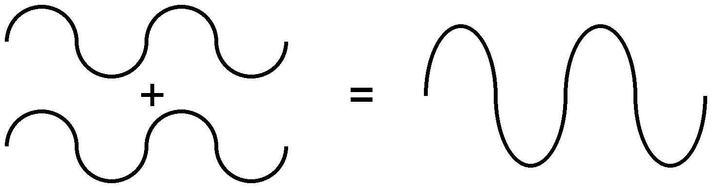
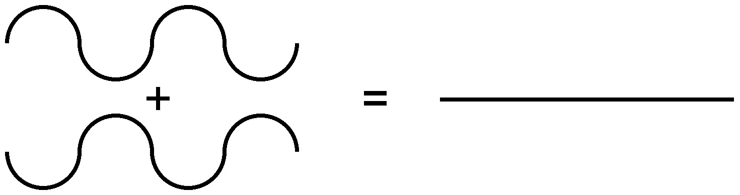
Because of the nature of diffraction, waves will experience either constructive (Figure \(\PageIndex{7}\)) or destructive (Figure \(\PageIndex{8}\)) interference with other waves. In the same way, when an X-ray beam is diffracted off a crystal, the different parts of the diffracted beam will have seemingly stronger energy, while other parts will have seemed to lost energy. This is dependent mostly on the wavelength of the incident beam, and the spacing between crystal lattices of the sample. Information about the lattice structure is obtained by varying beam wavelengths, incident angles, and crystal orientation. Much like solving a puzzle, a three dimensional structure of the crystalline solid can be constructed by observing changes in data with variation of the aforementioned variables.
The X-ray Diffractometer
At the heart of any XRD machine is the X-ray source. Modern day machines generally rely on copper metal as the element of choice for producing X-rays, although there are variations among different manufacturers. Because diffraction patterns are recorded over an extended period of time during sample analysis, it is very important that beam intensity remain constant throughout the entire analysis, or else faulty data will be procured. In light of this, even before an X-ray beam is generated, current must pass through a voltage regular, which will guarantee a steady stream of voltage to the X-ray source.
Another crucial component to the analysis of crystalline via X-rays is the detector. When XRD was first developed, film was the most commonly used method for recognizing diffraction patterns. The most obvious disadvantage to using film is the fact that it has to replaced every time a new specimen is introduced, making data collection a time consuming process. Furthermore, film can only be used once, leading to an increase in cost of operating diffraction analysis.
Since the origins of XRD, detection methods have progressed to the point where modern XRD machines are equipped with semiconductor detectors, which produce pulses proportional to the energy absorbed. With these modern detectors, there are two general ways in which a diffraction pattern may be obtained. The first is called continuous scan, and it is exactly what the name implies. The detector is set in a circular motion around the sample, while a beam of X-ray is constantly shot into the sample. Pulses of energy are plotted with respect to diffraction angle, which ensure all diffracted X-rays are recorded. The second and more widely used method is known as step scan. Step scanning bears similarity to continuous scan, except it is highly computerized and much more efficient. Instead of moving the detector in a circle around the entire sample, step scanning involves collecting data at one fixed angle at a time, thus the name. Within these detection parameters, the types of detectors can themselves be varied. A more common type of detector, known as the charge-coupled device (CCD) detector (Figure \(\PageIndex{9}\), can be found in many XRD machines, due to its fast data collection capability. A CCD detector is comprised of numerous radiation sensitive grids, each linked to sensors that measure changes in electromagnetic radiation. Another commonly seen type of detector is a simple scintillation counter (Figure \(\PageIndex{10}\)), which counts the intensity of X-rays that it encounters as it moves along a rotation axis. A comparable analogy to the differences between the two detectors mentioned would be that the CCD detector is able to see in two dimensions, while scintillation counters are only able to see in one dimension.
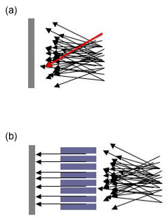
Aside from the above two components, there are many other variables involved in sample analysis by an XRD machine. As mentioned earlier, a steady incident beam is extremely important for good data collection. To further ensure this, there will often be what is known as a Söller slit or collimator found in many XRD machines. A Söller slit collimates the direction of the X-ray beam. In the collimated X-ray beam the rays are parallel, and therefore will spread minimally as they propagates (Figure \(\PageIndex{11}\). Without a collimator X-rays from all directions will be recorded; for example, a ray that has passed through the top of the specimen (see the red arrow in Figure \(\PageIndex{11}\)a) but happens to be traveling in a downwards direction may be recorded at the bottom of the plate. The resultant image will be so blurred and indistinct as to be useless. Some machines have a Söller slit between the sample and the detector, which drastically reduces the amount of background noise, especially when analyzing iron samples with a copper X-ray source.
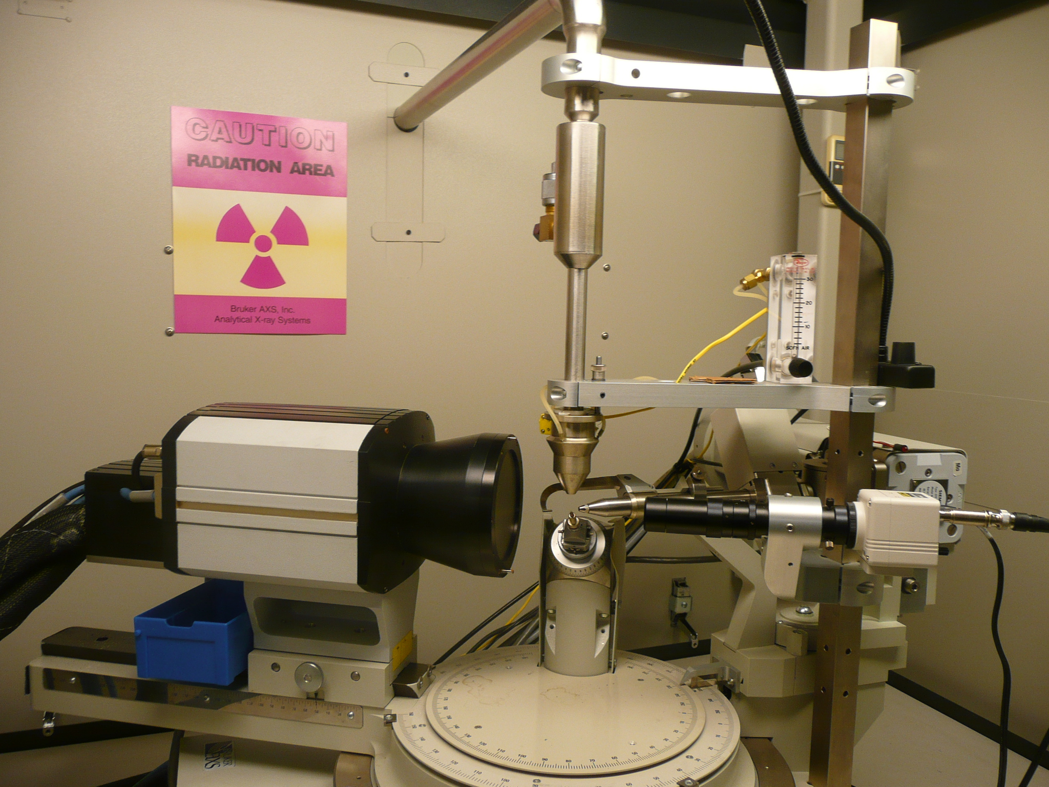
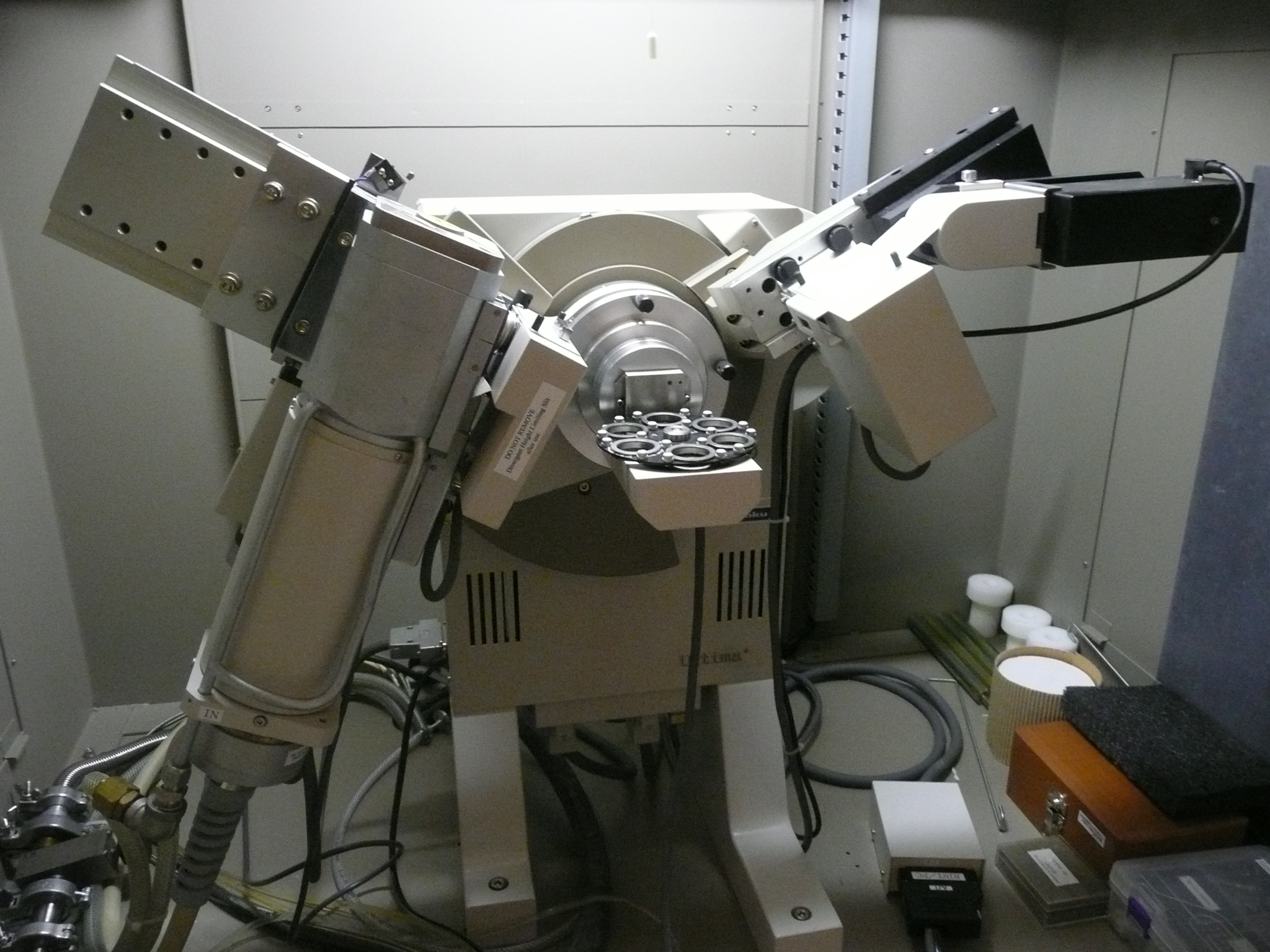
This single crystal XRD machine (Figure \(\PageIndex{12}\)) features a cooling gas line, which allows the user to bring down the temperature of a sample considerably below room temperature. Doing so allows for the opportunities for studies performed where the sample is kept in a state of extremely low energy, negating a lot of vibrational motion that might interfere with consistent data collection of diffraction patterns. Furthermore, information can be collected on the effects of temperature on a crystal structure. Also seen in Figure \(\PageIndex{13}\) is the hook-shaped object located between the beam emitter and detector. It serves the purpose of blocking X-rays that were not diffracted from being seen by the detector, drastically reducing the amount of unnecessary noise that would otherwise obscure data analysis.
Evolution of Powder XRD
Over time, XRD analysis has evolved from a very narrow and specific field to something that encompasses a much wider branch of the scientific arena. In its early stages, XRD was (with the exception of the simplest structures) confined to single crystal analysis, as detection methods had not advanced to a point where more complicated procedures was able to be performed. After many years of discovery and refining, however, technology has progressed to where crystalline properties (structure) of solids can be gleaned directly from a powder sample, thus offering information for samples that cannot be obtained as a single crystal. One area in which this is particularly useful is pharmaceuticals, since many of the compounds studied are not available in single crystal form, only in a powder.
Even though single crystal diffraction and powder diffraction essentially generate the same data, due to the powdered nature of the latter sample, diffraction lines will often overlap and interfere with data collection. This is apparently especially when the diffraction angle 2θ is high; patterns that emerge will be almost to the point of unidentifiable, because of disruption of individual diffraction patterns. For this particular reason, a new approach to interpreting powder diffraction data has been created.
There are two main methods for interpreting diffraction data:
- The first is known as the traditional method, which is very straightforward, and bears resemblance to single crystal data analysis. This method involves a two step process: 1) the intensities and diffraction patterns from the sample is collected, and 2) the data is analyzed to produce a crystalline structure. As mentioned before, however, data from a powdered sample is often obscured by multiple diffraction patterns, which decreases the chance that the generated structure is correct.
- The second method is called the direct-space approach. This method takes advantage of the fact that with current technology, diffraction data can be calculated for any molecule, whether or not it is the molecule in question. Even before the actual diffraction data is collected, a large number of theoretical patterns of suspect molecules are generated by computer, and compared to experimental data. Based on correlation and how well the theoretical pattern fits the experimental data best, a guess is formulated to which compound is under question. This method has been taken a step further to mimic social interactions in a community. For example, first generation theoretical trial molecules, after comparison with the experimental data, are allowed to evolve within parameters set by researchers. Furthermore, if appropriate, molecules are produce offspring with other molecules, giving rise to a second generation of molecules, which fit the experimental data even better. Just like a natural environment, genetic mutations and natural selection are all introduced into the picture, ultimately giving rise a molecular structure that represents data collected from XRD analysis.
Another important aspect of being able to study compounds in powder form for the pharmaceutical researcher is the ability to identify structures in their natural state. A vast majority of drugs in this day and age are delivered through powdered form, either in the form of a pill or a capsule. Crystallization processes may often alter the chemical composition of the molecule (e.g., by the inclusion of solvent molecules), and thus marring the data if confined to single crystal analysis. Furthermore, when the sample is in powdered form, there are other variables that can be adjusted to see real-time effects on the molecule. Temperature, pressure, and humidity are all factors that can be changed in-situ to glean data on how a drug might respond to changes in those particular variables.
Powder X-Ray Diffraction
Introduction
Powder X-Ray diffraction (XRD) was developed in 1916 by Debye (Figure \(\PageIndex{12}\)) and Scherrer (Figure \(\PageIndex{13}\)) as a technique that could be applied where traditional single-crystal diffraction cannot be performed. This includes cases where the sample cannot be prepared as a single crystal of sufficient size and quality. Powder samples are easier to prepare, and is especially useful for pharmaceuticals research.
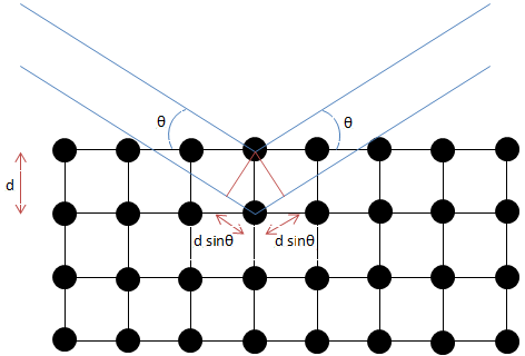
Diffraction occurs when a wave meets a set of regularly spaced scattering objects, and its wavelength of the distance between the scattering objects are of the same order of magnitude. This makes X-rays suitable for crystallography, as its wavelength and crystal lattice parameters are both in the scale of angstroms (Å). Crystal diffraction can be described by Bragg diffraction, \ref{2}, where λ is the wavelength of the incident monochromatic X-ray, d is the distance between parallel crystal planes, and θ the angle between the beam and the plane.
\[ \lambda \ =\ 2d\ sin \theta \label{2} \]
For constructive interference to occur between two waves, the path length difference between the waves must be an integral multiple of their wavelength. This path length difference is represented by 2d sinθ Figure \(\PageIndex{14}\). Because sinθ cannot be greater than 1, the wavelength of the X-ray limits the number of diffraction peaks that can appear.
Production and Detection of X-rays
Most diffractometers use Cu or Mo as an X-ray source, and specifically the Kα radiation of wavelengths of 1.54059 Å and 0.70932 Å, respectively. A stream of electrons is accelerated towards the metal target anode from a tungsten cathode, with a potential difference of about 30-50 kV. As this generates a lot of heat, the target anode must be cooled to prevent melting.
Detection of the diffracted beam can be done in many ways, and one common system is the gas proportional counter (GPC). The detector is filled with an inert gas such as argon, and electron-ion pairs are created when X-rays pass through it. An applied potential difference separates the pairs and generates secondary ionizations through an avalanche effect. The amplification of the signal is necessary as the intensity of the diffracted beam is very low compared to the incident beam. The current detected is then proportional to the intensity of the diffracted beam. A GPC has a very low noise background, which makes it widely used in labs.
Performing X-ray Diffraction
Exposure to X-rays may have health consequences, follow safety procedures when using the diffractometer.
The particle size distribution should be even to ensure that the diffraction pattern is not dominated by a few large particles near the surface. This can be done by grinding the sample to reduce the average particle size to <10µm. However, if particle sizes are too small, this can lead to broadening of peaks. This is due to both lattice damage and the reduction of the number of planes that cause destructive interference.
The diffraction pattern is actually made up of angles that did not suffer from destructive interference due to their special relationship described by Bragg Law (Figure \(\PageIndex{15}\)). If destructive interference is reduced close to these special angles, the peak is broadened and becomes less distinct. Some crystals such as calcite (CaCO3, Figure \(\PageIndex{15}\) have preferred orientations and will change their orientation when pressure is applied. This leads to differences in the diffraction pattern of ‘loose’ and pressed samples. Thus, it is important to avoid even touching ‘loose’ powders to prevent errors when collecting data.
The sample powder is loaded onto a sample dish for mounting in the diffractometer (Figure \(\PageIndex{16}\)), where rotating arms containing the X-ray source and detector scan the sample at different incident angles. The sample dish is rotated horizontally during scanning to ensure that the powder is exposed evenly to the X-rays.

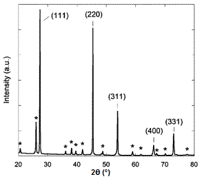
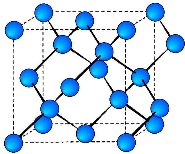
A sample X-ray diffraction spectrum of germanium is shown in Figure \(\PageIndex{17}\), with peaks identified by the planes that caused that diffraction. Germanium has a diamond cubic crystal lattice (Figure \(\PageIndex{18}\)), named after the crystal structure of prototypical example. The crystal structure determines what crystal planes cause diffraction and the angles at which they occur. The angles are shown in 2θ as that is the angle measured between the two arms of the diffractometer, i.e., the angle between the incident and the diffracted beam (Figure \(\PageIndex{14}\)).
Determining Crystal Structure for Cubic Lattices
There are three basic cubic crystal lattices, and they are the simple cubic (SC), body-centered cubic (BCC), and the face-centered cubic (FCC) Figure \(\PageIndex{19}\). These structures are simple enough to have their diffraction spectra analyzed without the aid of software.
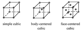
Each of these structures has specific rules on which of their planes can produce diffraction, based on their Miller indices (hkl).
- SC lattices show diffraction for all values of (hkl), e.g., (100), (110), (111), etc.
- BCC lattices show diffraction when the sum of h+k+l is even, e.g., (110), (200), (211), etc.
- FCC lattices show diffraction when the values of (hkl) are either all even or all odd, e.g., (111), (200), (220), etc.
- Diamond cubic lattices like that of germanium are FCC structures with four additional atoms in the opposite corners of the tetrahedral interstices. They show diffraction when the values of (hkl) are all odd or all even and the sum h+k+l is a multiple of 4, e.g., (111), (220), (311), etc.
The order in which these peaks appear depends on the sum of h2+k2+l2. These are shown in Table \(\PageIndex{1}\).
| (hkl) | h2+k2+l2 | BCC | FCC |
| 100 | 1 | ||
| 110 | 2 | Y | |
| 111 | 3 | Y | |
| 200 | 4 | Y | Y |
| 210 | 5 | ||
| 211 | 6 | Y | |
| 220 | 8 | Y | Y |
| 300, 221 | 9 | ||
| 310 | 10 | Y | |
| 311 | 11 | Y | |
| 222 | 12 | Y | Y |
| 320 | 13 | ||
| 321 | 14 | Y | |
| 400 | 16 | Y | Y |
| 410, 322 | 17 | ||
| 411, 330 | 18 | Y | |
| 331 | 19 | Y | |
| 420 | 20 | Y | Y |
| 421 | 21 |
The value of d for each of these planes can be calculated using \ref{3}, where a is the lattice parameter of the crystal.
The lattice constant, or lattice parameter, refers to the constant distance between unit cells in a crystal lattice.
\[ \frac{1}{d^{2}} \ =\ \frac{h^{2}+k^{2}+l^{2}}{a^{2}} \label{3} \]
As the diamond cubic structure of Ge can be complicated, a simpler worked example for sample diffraction of NaCl with Cu-Kα radiation is shown below. Given the values of 2θ that result in diffraction, Table \(\PageIndex{2}\) can be constructed.
| 2θ | θ | Sinθ | Sin2θ |
| 27.36 | 13.68 | 0.24 | 0.0559 |
| 31.69 | 15.85 | 0.27 | 0.0746 |
| 45.43 | 22.72 | 0.39 | 0.1491 |
| 53.85 | 26.92 | 0.45 | 0.2050 |
| 56.45 | 28.23 | 0.47 | 0.2237 |
| 66.20 | 33.10 | 0.55 | 0.2982 |
| 73.04 | 36.52 | 0.60 | 0.3541 |
| 75.26 | 37.63 | 0.61 | 0.3728 |
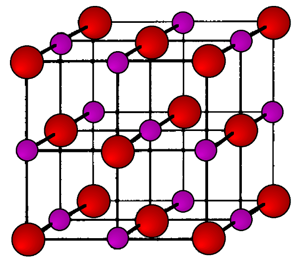
The values of these ratios can then be inspected to see if they corresponding to an expected series of hkl values. In this case, the last column gives a list of integers, which corresponds to the h2+k2+l2 values of the FCC lattice diffraction. Hence, NaCl has a FCC structure, shown in angles Figure \(\PageIndex{20}\).
The lattice parameter of NaCl can now be calculated from this data. The first peak occurs at θ = 13.68°. Given that the wavelength of the Cu-Kα radiation is 1.54059 Å, Bragg's Equation \ref{4} can be applied as follows:
\[ 1.54059 \ =\ 2d\ sin 13.68 \label{4} \]
\[ d\ =\ 3.2571\ Å \label{5} \]
Since the first peak corresponds to the (111) plane, the distance between two parallel (111) planes is 3.2571 Å. The lattice parameter can now be worked out using \ref{6}.
\[ 1/3.2561^{2}\ =\ (1^{2}+1^{2}+I^{2})/a^{2} \label{6} \]
\[ a\ =\ 5.6414\ Å \label{7} \]
The powder XRD spectrum of Ag nanoparticles is given in Figure \(\PageIndex{21}\) as collected using Cu-Kα radiation of 1.54059 Å. Determine its crystal structure and lattice parameter using the labeled peaks.
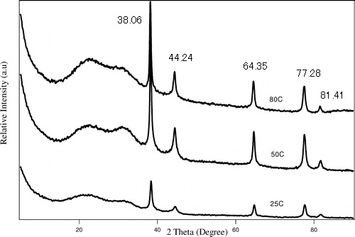
| 2θ | θ | Sinθ | Sin2θ | Sin2θ/Sin2θ | 2 x Sin2θ/Sin2θ | 3 x Sin2θ/Sin2θ |
| 38.06 | 19.03 | 0.33 | 0.1063 | 1.00 | 2.00 | 3.00 |
| 44.24 | 22.12 | 0.38 | 0.1418 | 1.33 | 2.67 | 4.00 |
| 64.35 | 32.17 | 0.53 | 0.2835 | 2.67 | 5.33 | 8 |
| 77.28 | 38.64 | 0.62 | 0.3899 | 3.67 | 7.34 | 11 |
| 81.41 | 40.71 | 0.65 | 0.4253 | 4 | 8 | 12 |
| 97.71 | 48.86 | 0.75 | 0.5671 | 5.33 | 10.67 | 16 |
| 110.29 | 55.15 | 0.82 | 0.6734 | 6.34 | 12.67 | 19.01 |
| 114.69 | 57.35 | 0.84 | 0.7089 | 6.67 | 13.34 | 20.01 |
Applying the Bragg Equation \ref{8},
\[ 1.54059\ =\ 2d\ sin\ 19.03 \label{8} \]
\[ d\ =\ 2.3624\ Å \label{9} \]
Calculate the lattice parameter using \ref{10},
\[ 1/2.3624^{2}\ =\ (1^{2}+1^{2}+I^{2})/a^{2} \label{10} \]
\[ a\ =\ 4.0918\ Å \label{11} \]
The last column gives a list of integers, which corresponds to the h2+k2+l2 values of the FCC lattice diffraction. Hence, the Ag nanoparticles have a FCC structure.
Determining Composition
As seen above, each crystal will give a pattern of diffraction peaks based on its lattice type and parameter. These fingerprint patterns are compiled into databases such as the one by the Joint Committee on Powder Diffraction Standard (JCPDS). Thus, the XRD spectra of samples can be matched with those stored in the database to determine its composition easily and rapidly.
Solid State Reaction Monitoring
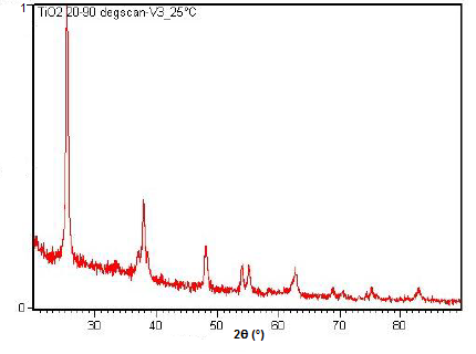
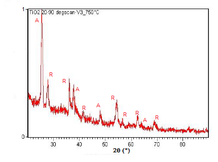
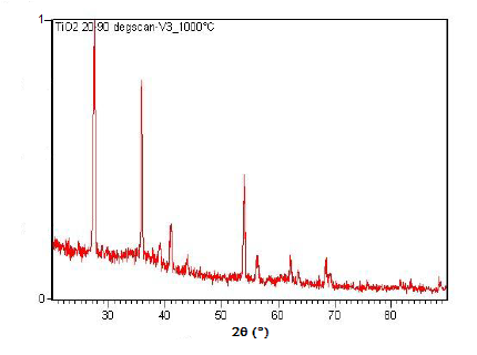
Powder XRD is also able to perform analysis on solid state reactions such as the titanium dioxide (TiO2) anatase to rutile transition. A diffractometer equipped with a sample chamber that can be heated can take diffractograms at different temperatures to see how the reaction progresses. Spectra of the change in diffraction peaks during this transition is shown in Figure \(\PageIndex{22}\), Figure \(\PageIndex{23}\), and Figure \(\PageIndex{24}\).
Summary
XRD allows for quick composition determination of unknown samples and gives information on crystal structure. Powder XRD is a useful application of X-ray diffraction, due to the ease of sample preparation compared to single-crystal diffraction. Its application to solid state reaction monitoring can also provide information on phase stability and transformation.
An Introduction to Single-Crystal X-Ray Crystallography
Described simply, single-crystal X-ray diffraction (XRD) is a technique in which a crystal of a sample under study is bombarded with an X-ray beam from many different angles, and the resulting diffraction patterns are measured and recorded. By aggregating the diffraction patterns and converting them via Fourier transform to an electron density map, a unit cell can be constructed which indicates the average atomic positions, bond lengths, and relative orientations of the molecules within the crystal.
Fundamental Principles
As an analogy to describe the underlying principles of diffraction, imagine shining a laser onto a wall through a fine sieve. Instead of observing a single dot of light on the wall, a diffraction pattern will be observed, consisting of regularly arranged spots of light, each with a definite position and intensity. The spacing of these spots is inversely related to the grating in the sieve— the finer the sieve, the farther apart the spots are, and the coarser the sieve, the closer together the spots are. Individual objects can also diffract radiation if it is of the appropriate wavelength, but a diffraction pattern is usually not seen because its intensity is too weak. The difference with a sieve is that it consists of a grid made of regularly spaced, repeating wires. This periodicity greatly magnifies the diffraction effect because of constructive interference. As the light rays combine amplitudes, the resulting intensity of light seen on the wall is much greater because intensity is proportional to the square of the light’s amplitude.
To apply this analogy to single-crystal XRD, we must simply scale it down. Now the sieve is replaced by a crystal and the laser (visible light) is replaced by an X-ray beam. Although the crystal appears solid and not grid-like, the molecules or atoms contained within the crystal are arranged periodically, thus producing the same intensity-magnifying effect as with the sieve. Because X-rays have wavelengths that are on the same scale as the distance between atoms, they can be diffracted by their interactions with the crystal lattice.
These interactions are dictated by Bragg's law, which says that constructive interference occurs only when \ref{12} is satisfied; where n is an integer, λ is the wavelength of light, d is the distance between parallel planes in the crystal lattice, and θ is the angle of incidence between the X-ray beam and the diffracting planes (see Figure \(\PageIndex{25}\)). A complication arises, however, because crystals are periodic in all three dimensions, while the sieve repeats in only two dimensions. As a result, crystals have many different diffraction planes extending in certain orientations based on the crystal’s symmetry group. For this reason, it is necessary to observe diffraction patterns from many different angles and orientations of the crystal to obtain a complete picture of the reciprocal lattice.
The reciprocal lattice of a lattice (Bravais lattice) is the lattice in which the Fourier transform of the spatial wavefunction of the original lattice (or direct lattice) is represented. The reciprocal lattice of a reciprocal lattice is the original lattice.
\[ n \lambda \ =\ 2d\ sin \theta \label{12} \]
The reciprocal lattice is related to the crystal lattice just as the sieve is related to the diffraction pattern: they are inverses of each other. Each point in real space has a corresponding point in reciprocal space and they are related by 1/d; that is, any vector in real space multiplied by its corresponding vector in reciprocal space gives a product of unity. The angles between corresponding pairs of vectors remains unchanged.
Real space is the domain of the physical crystal, i.e. it includes the crystal lattice formed by the physical atoms within the crystal. Reciprocal space is, simply put, the Fourier transform of real space; practically, we see that diffraction patterns resulting from different orientations of the sample crystal in the X-ray beam are actually two-dimensional projections of the reciprocal lattice. Thus by collecting diffraction patterns from all orientations of the crystal, it is possible to construct a three-dimensional version of the reciprocal lattice and then perform a Fourier transform to model the real crystal lattice.
Technique
Single-crystal Versus Powder Diffraction
Two common types of X-ray diffraction are powder XRD and single-crystal XRD, both of which have particular benefits and limitations. While powder XRD has a much simpler sample preparation, it can be difficult to obtain structural data from a powder because the sample molecules are randomly oriented in space; without the periodicity of a crystal lattice, the signal-to-noise ratio is greatly decreased and it becomes difficult to separate reflections coming from the different orientations of the molecule. The advantage of powder XRD is that it can be used to quickly and accurately identify a known substance, or to verify that two unknown samples are the same material.
Single-crystal XRD is much more time and data intensive, but in many fields it is essential for structural determination of small molecules and macromolecules in the solid state. Because of the periodicity inherent in crystals, small signals from individual reflections are magnified via constructive interference. This can be used to determine exact spatial positions of atoms in molecules and can yield bond distances and conformational information. The difficulty of single-crystal XRD is that single crystals may be hard to obtain, and the instrument itself may be cost-prohibitive.
An example of typical diffraction patterns for single-crystal and powder XRD follows ((Figure \(\PageIndex{27}\) and Figure \(\PageIndex{28}\), respectively). The dots in the first image correspond to Bragg reflections and together form a single view of the molecule’s reciprocal space. In powder XRD, random orientation of the crystals means reflections from all of them are seen at once, producing the observed diffraction rings that correspond to particular vectors in the material’s reciprocal lattice.
Technique
In a single-crystal X-ray diffraction experiment, the reciprocal space of a crystal is constructed by measuring the angles and intensities of reflections in observed diffraction patterns. These data are then used to create an electron density map of the molecule which can be refined to determine the average bond lengths and positions of atoms in the crystal.
Instrumentation
The basic setup for single-crystal XRD consist of an X-ray source, a collimator to focus the beam, a goniometer to hold and rotate the crystal, and a detector to measure and record the reflections. Instruments typically contain a beamstop to halt the primary X-ray beam from hitting the detector, and a camera to help with positioning the crystal. Many also contain an outlet connected to a cold gas supply (such as liquid nitrogen) in order to cool the sample crystal and reduce its vibrational motion as data is being collected. A typical instrument is shown in Figure \(\PageIndex{28}\) and Figure \(\PageIndex{31}\).
Obtaining Single Crystals
Despite advances in instrumentation and computer programs that make data collection and solving crystal structures significantly faster and easier, it can still be a challenge to obtain crystals suitable for analysis. Ideal crystals are single, not twinned, clear, and of sufficient size to be mounted within the the X-ray beam (usually 0.1-0.3 mm in each direction). They also have clean faces and smooth edges. Following are images of some ideal crystals (Figure \(\PageIndex{30}\) and Figure \(\PageIndex{31}\)), as well as an example of twinned crystals (Figure \(\PageIndex{32}\)).
Crystal twinning occurs when two or more crystals share lattice points in a symmetrical manner. This usually results in complex diffraction patterns which are difficult to analyze and construct a reciprocal lattice.
Crystal formation can be affected by temperature, pressure, solvent choice, saturation, nucleation, and substrate. Slow crystal growth tends to be best, as rapid growth creates more imperfections in the crystal lattice and may even lead to a precipitate or gel. Similarly, too many nucleation sites (points at which crystal growth begins) can lead to many small crystals instead of a few, well-defined ones.
There are a number of basic methods for growing crystals suitable for single-crystal XRD:
- The most basic method is to slowly evaporate a saturated solution until it becomes supersaturated and then forms crystals. This often works well for growing small-molecule crystals; macroscopic molecules (such as proteins) tend to be more difficult.
- A solution of the compound to be crystallized is dissolved in one solvent, then a ‘non-solvent’ which is miscible with the first but in which the compound itself is insoluble, is carefully layered on top of the solution. As the non-solvent mixes with the solvent by diffusion, the solute molecules are forced out of solution and may form crystals.
- A crystal solution is placed in a small open container which is then set in a larger closed container holding a volatile non-solvent. As the volatile non-solvent mixes slowly with the solution by vapor diffusion, the solute is again forced to come out of solution, often leading to crystal growth.
- All three of the previous techniques can be combined with seeding, where a crystal of the desired type to be grown is placed in the saturated solution and acts as a nucleation site and starting place for the crystal growth to begin. In some cases, this can even cause crystals to grow in a form that they would not normally assume, as the seed can act as a template that might not otherwise be followed.
- The hanging drop technique is typically used for growing protein crystals. In this technique, a drop of concentrated protein solution is suspended (usually by dotting it on a silicon-coated microscope slide) over a larger volume of the solution. The whole system is then sealed and slow evaporation of the suspended drop causes it to become supersaturated and form crystals. (A variation of this is to have the drop of protein solution resting on a platform inside the closed system instead of being suspended from the top of the container.)
These are only the most common ways that crystals are grown. Particularly for macromolecules, it may be necessary to test hundreds of crystallization conditions before a suitable crystal is obtained. There now exist automated techniques utilizing robots to grow crystals, both for obtaining large numbers of single crystals and for performing specialized techniques (such as drawing a crystal out of solution) that would otherwise be too time-consuming to be of practical use.
Wide Angle X-ray Diffraction Studies of Liquid Crystals
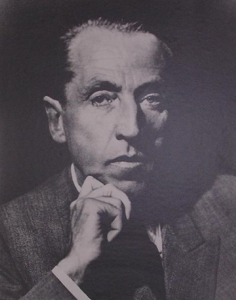
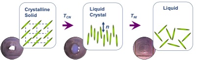
Some organic molecules display a series of intermediate transition states between solid and isotropic liquid states (Figure \(\PageIndex{33}\)) as their temperature is raised. These intermediate phases have properties in between the crystalline solid and the corresponding isotropic liquid state, and hence they are called liquid crystalline phases. Other name is mesomorphic phases where mesomorphic means of intermediate form. According to the physicist de Gennes (Figure \(\PageIndex{34}\)), liquid crystal is ‘an intermediate phase, which has liquid like order in at least one direction and possesses a degree of anisotropy’. It should be noted that all liquid crystalline phases are formed by anisotropic molecules (either elongated or disk-like) but not all the anisotropic molecules form liquid crystalline phases.

Anisotropic objects can possess different types of ordering giving rise to different types of liquid crystalline phases (Figure \(\PageIndex{35}\)).
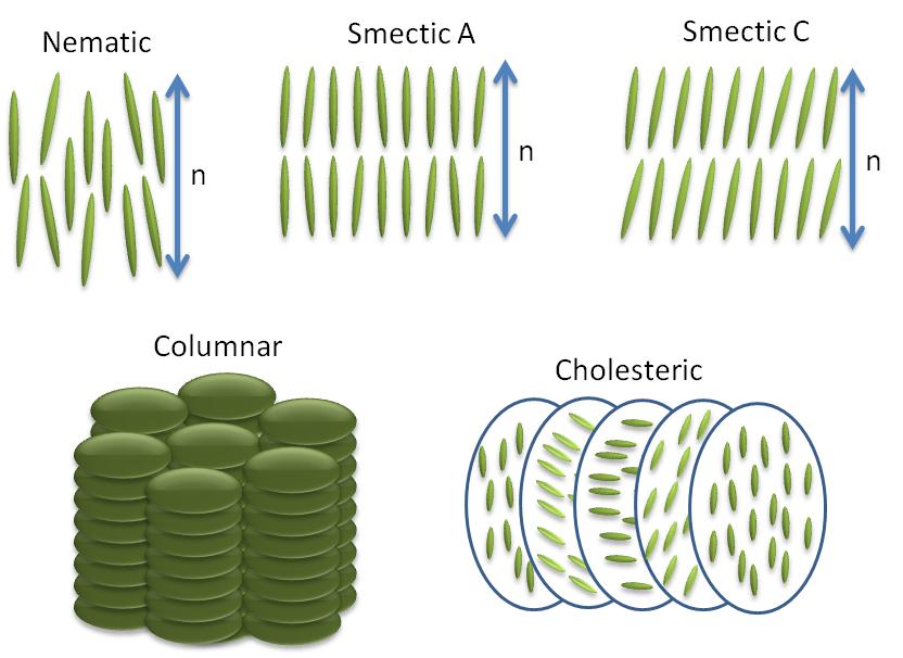
Nematic Phases
The word nematic comes from the Greek for thread, and refers to the thread-like defects commonly observed in the polarizing optical microscopy of these molecules. They have no positional order only orientational order, i.e., the molecules all pint in the same direction. The direction of molecules denoted by the symbol n commonly referred as the ‘director’ (Figure \(\PageIndex{36}\)). The director n is bidirectional that means the states n and -n are indistinguishable.
Smetic Phases
All the smectic phases are layered structures that usually occur at slightly lower temperatures than nematic phases. There are many variations of smectic phases, and some of the distinct ones are as follows:
- Each layer in smectic A is like a two dimensional liquid, and the long axis of the molecules is typically orthogonal to the layers (Figure \(\PageIndex{35}\).
- Just like nematics, the state n and -n are equivalent. They are made up of achiral and non polar molecules.
- As with smectic A, the smectic C phase is layered, but the long axis of the molecules is not along the layers normal. Instead it makes an angle (θ, Figure \(\PageIndex{35}\)). The tilt angle is an order parameter of this phase and can vary from 0° to 45-50°.
- Smectic C* phases are smectic phases formed by chiral molecules. This added constraint of chirality causes a slight distortion of the Smectic C structure. Now the tilt direction precesses around the layer normal and forms a helical configuration.
Cholesterics Phases
Sometimes cholesteric phases (Figure \(\PageIndex{35}\)) are also referred to as chiral nematic phases because they are similar to nematic phases in many regards. Many derivatives of cholesterol exhibit this type of phase. They are generally formed by chiral molecules or by doping the nematic host matrix with chiral molecules. Adding chirality causes helical distortion in the system, which makes the director, n, rotate continuously in space in the shape of a helix with specific pitch. The magnitude of pitch in a cholesteric phase is a strong function of temperature.
Columnar Phases
In columnar phases liquid crystals molecules are shaped like disks as opposed to rod-like in nematic and smectics liquid crystal phases. These disk shaped molecules stack themselves in columns and form a 2D crystalline array structures (Figure \(\PageIndex{35}\)). This type of two dimensional ordering leads to new mesophases.
Introduction to 2D X-ray Diffraction
X-ray diffraction (XRD) is one of the fundamental experimental techniques used to analyze the atomic arrangement of materials. The basic principle behind X-ray diffraction is Bragg’s Law (Figure \(\PageIndex{36}\)). According to this law, X-rays that are reflected from the adjacent crystal planes will undergo constructive interference only when the path difference between them is an integer multiple of the X-ray's wavelength, \ref{13}, where n is an integer, d is the spacing between the adjacent crystal planes, θ is the angle between incident X-ray beam and scattering plane, and λ is the wavelength of incident X-ray.
\[ 2d sin \theta \ =\ n \lambda \label{13}\ \]
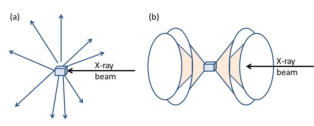
Now the atomic arrangement of molecules can go from being extremely ordered (single crystals) to random (liquids). Correspondingly, the scattered X-rays form specific diffraction patterns particular to that sample. Figure \(\PageIndex{37}\) shows the difference between X-rays scattered from a single crystal and a polycrystalline (powder) sample. In case of a single crystal the diffracted rays point to discrete directions (Figure \(\PageIndex{37}a\)), while for polycrystalline sample diffracted rays form a series of diffraction cones (Figure \(\PageIndex{37}b\)).
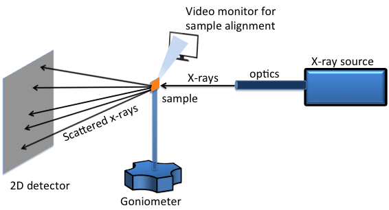
A two dimensional (2D) XRD system is a diffraction system with the capability of simultaneously collecting and analyzing the X-ray diffraction pattern in two dimensions. A typical 2D XRD setup consists of five major components (Figure \(\PageIndex{38}\)):
- X-ray source.
- X-ray optics.
- Goniometer.
- Sample alignment and monitoring device.
- 2D area detector.
For laboratory scale X-ray generators, X-rays are emitted by bombarding metal targets with high velocity electrons accelerated by strong electric field in the range 20-60 kV. Different metal targets that can be used are chromium (Cr), cobalt (Co), copper (Cu), molybdenum (Mo) and iron (Fe). The most commonly used ones are Cu and Mo. Synchrotrons are even higher energy radiation sources. They can be tuned to generate a specific wavelength and they have much brighter luminosity for better resolution. Available synchrotron facilities in US are:
- Stanford Synchrotron Radiation Lightsource (SSRL), Stanford, CA.
- Synchrotron Radiation Center (SRC), University of Wisconsin-Madison, Madison, WI.
- Advanced Light Source (ALS), Lawrence Berkeley National, Berkeley, CA.
- National Synchrotron Light Source (NSLS), Brookhaven National Laboratory, Upton, NY.
- Advanced Photon Source (APS), Argonne National Laboratory, Argonne, IL.
- Center for Advanced Microstructures & Devices, Louisiana State University, Baton Rouge, LA.
- Cornell High Energy Synchrotron Source (CHESS), Cornell, Ithaca, NY.
The X-ray optics are comprised of the X-ray tube, monochromator, pinhole collimator and beam stop. A monochromator is used to get rid of unwanted X-ray radiation from the X-ray tube. A diffraction from a single crystal can be used to select a specific wavelength of radiation. Typical materials used are pyrolytic graphite and silicon. Monochromatic X-ray beams have three components: parallel, convergent and divergent X-rays. The function of a pinhole collimator is to filter the incident X-ray beam and allow passage of parallel X-rays. A 2D X-ray detector can either be a film or a digital detector, and its function is to measure the intensity of X-rays diffracted from a sample as a function of position, time, and energy.
Advantages of 2D XRD as Compared to 1D XRD
2D diffracton data has much more information in comparison diffraction pattern, which is acquired using a 1D detector. Figure \(\PageIndex{39}\) shows the diffraction pattern from a polycrystalline sample. For illustration purposes only, two diffraction cones are shown in the schematic. In the case of 1D X-ray diffraction, measurement area is confined within a plane labeled as diffractometer plane. The 1D detector is mounted along the detection circle and variation of diffraction pattern in the z direction are not considered. The diffraction pattern collected is an average over a range defined by a beam size in the z direction. The diffraction pattern measured is a plot of X-ray intensity at different 2θ angles. For 2D X-ray diffraction, the measurement area is not limited to the diffractometer plane. Instead, a large portion of the diffraction rings are measured simultaneously depending on the detector size and position from the sample.
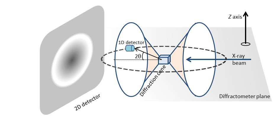
One such advantage is the measurement of percent crystallinity of a material. Determination of material crystallinity is required both for research and quality control. Scattering from amorphous materials produces a diffuse intensity ring while polycrystalline samples produce sharp and well-defined rings or spots are seen. The ability to distinguish between amorphous and crystalline is the key in determining percent of crystallinity accurately. Since most crystalline samples have preferred orientation, depending on the sample is oriented it is possible to measure different peak or no peak using conventional diffraction system. On the other hand, sample orientation has no effect on the full circle integrated diffraction measuring done using 2D detector. A 2D XRD can therefore measure percent crystallinity more accurately.
2D Wide Angle X-ray Diffraction Patterns of LCs
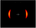
As mentioned in the introduction section, liquid crystal is an intermediate state between solid and liquid phases. At temperatures above the liquid crystal phase transition temperature (Figure \(\PageIndex{40}\)), they become isotropic liquid, i.e., absence of long-range positional or orientational order within molecules. Since an isotropic state cannot be aligned, its diffraction pattern consists of weak, diffuse rings Figure \(\PageIndex{40}a\). The reason we see any diffraction pattern in the isotropic state is because in classical liquids there exists a short range positional order. The ring has of radius of 4.5 Å and it mostly appears at 20.5°. It represents the distance between the molecules along their widths.
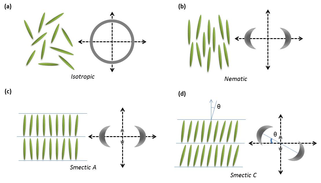
Nematic liquid crystalline phases have long range orientational order but no positional order. An unaligned sample of nematic liquid crystal has similar diffraction pattern as an isotropic state. But instead of a diffuse ring, it has a sharper intensity distribution. For an aligned sample of nematic liquid crystal, X-ray diffraction patterns exhibit two sets of diffuse arcs (Figure \(\PageIndex{40}\) b). The diffuse arc at the larger radius (P1, 4.5 Å) represents the distance between molecules along their widths. Under the presence of an external magnetic field, samples with positive diamagnetic anisotropy align parallel to the field and P1 is oriented perpendicularly to the field. While samples with negative diamagnetic anisotropy align perpendicularly to the field with P1 being parallel to the field. The intensity distribution within these arcs represents the extent of alignment within the sample; generally denoted by S.
The diamagnetic anistropy of all liquid crystals with an aromatic ring is positive, and on order of 10-7. The value decreases with the substitution of each aromatic ring by a cyclohexane or other aliphatic group. A negative diamagnetic anistropy is observed for purely cycloaliphatic LCs.
When a smectic phase is cooled down slowly under the presence the external field, two sets of diffuse peaks are seen in diffraction pattern (Figure \(\PageIndex{40}\) c). The diffuse peak at small angles condense into sharp quasi-Bragg peaks. The peak intensity distribution at large angles is not very sharp because molecules within the smectic planes are randomly arranged. In case of smectic C phases, the angle between the smectic layers normal and the director (θ) is no longer collinear (Figure \(\PageIndex{40}\) d). This tilt can easily be seen in the diffraction pattern as the diffuse peaks at smaller and larger angles are no longer orthogonal to each other.
Sample Preparation
In general, X-ray scattering measurements of liquid crystal samples are considered more difficult to perform than those of crystalline samples. The following steps should be performed for diffraction measurement of liquid crystal samples:
- The sample should be free of any solvents and absorbed oxygen, because their presence affects the liquid crystalline character of the sample and its thermal response. This can be achieved by performing multiple melting and freezing cycles in a vacuum to get rid of unwanted solvents and gases.
- For performing low resolution measurements, liquid crystal sample can be placed inside a thin-walled glass capillary. The ends of the capillary can be sealed by epoxy in case of volatile samples. The filling process tends to align the liquid crystal molecules along the flow direction.
- For high resolution measurements, the sample is generally confined between two rubbed polymer coated glass coverslips separated by an o-ring as a spacer. The rubbing causes formation of grooves in the polymer film which tends to the align the liquid crystal molecules.
- Aligned samples are necessary for identifying the liquid crystalline phase of the sample. Liquid crystal samples can be aligned by heating above the phase transition temperature and cooling them slowly in the presence of an external electric or magnetic field. A magnetic field is effective for samples with aromatic cores as they have high diamagnetic anisotropy. A common problem in using electric field is internal heating which can interfere with the measurement.
- Sample size should be sufficient to avoid any obstruction to the passage of the incident X-ray beam.
- The sample thickness should be around one absorption length of the X-rays. This allows about 63% of the incident light to pass through and get optimum scattering intensity. For most hydrocarbons absorption length is approximately 1.5 mm with a copper metal target (λ = 1.5418 Å). Molybdenum target can be used for getting an even higher energy radiation (λ = 0.71069 Å ).
Data Analysis
Identification of the phase of a liquid crystal sample is critical in predicting its physical properties. A simple 2D X-ray diffraction pattern can tell a lot in this regard (Figure \(\PageIndex{40}\)). It is also critical to determine the orientational order of a liquid crystal. This is important to characterize the extent of sample alignment.
For simplicity, the rest of the discussion focuses on nematic liquid crystal phases. In an unaligned sample, there isn't any specific macroscopic order in the system. In the micrometer size domains, molecules are all oriented in a specific direction, called a local director. Because there is no positional order in nematic liquid crystals, this local director varies in space and assumes all possible orientations. For example, in a perfectly aligned sample of nematic liquid crystals, all the local directors will be oriented in the same direction. The specific alignment of molecules in one preferred direction in liquid crystals makes their physical properties such as refractive index, viscosity, diamagnetic susceptibility, directionally dependent.
When a liquid crystal sample is oriented using external fields, local directors preferentially align globally along the field director. This globally preferred direction is referred to as the director and is denoted by unit vector n. The extent of alignment within a liquid crystal sample is typically denoted by the order parameter, S, as defined by \ref{14}, where θ is the angle between long axis of molecule and the preferred direction, n.
\[ S\ =\ (\frac{3cos^{2} \theta \ -\ 1}{2}) \label{14} \]
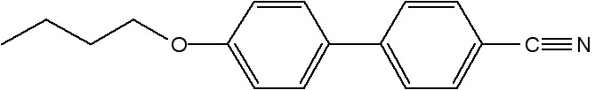
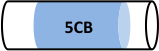
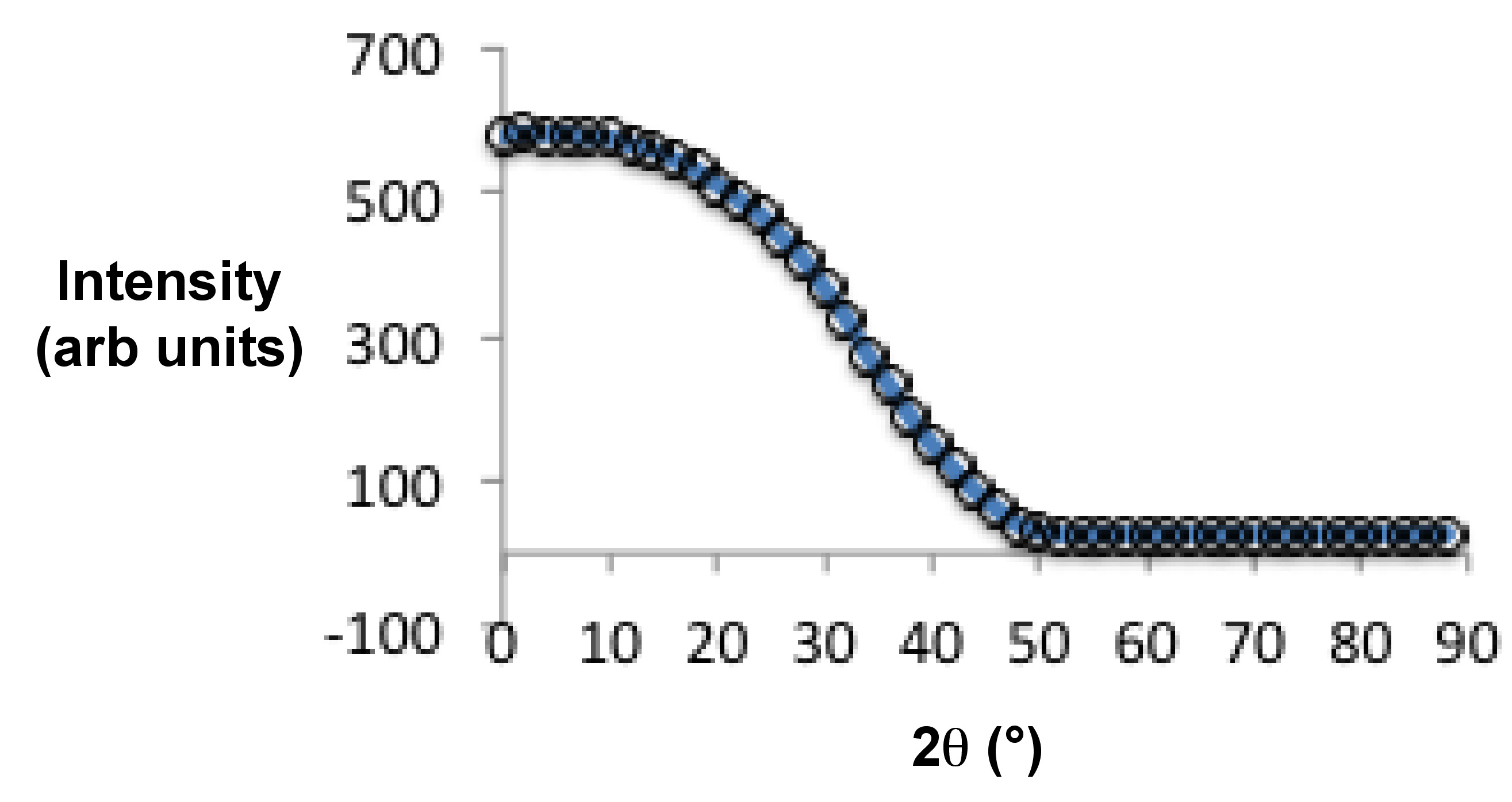
For isotropic samples, the value of S is zero, and for perfectly aligned samples it is 1. Figure \(\PageIndex{41}\) shows the structure of a most extensively studied nematic liquid crystal molecule, 4-cyano-4'-pentylbiphenyl, commonly known as 5CB. For preparing a polydomain sample 5CB was placed inside a glass capillary via capillary forces (Figure \(\PageIndex{41}\)). Figure \(\PageIndex{42}\) shows the 2D X-ray diffraction of the as prepared polydomain sample. For preparing monodomain sample, a glass capillary filled with 5CB was heated to 40 °C (i.e., above the nematic-isotropic transition temperature of 5CB, ~35 °C) and then cooled slowly in the presence of magnetic field (1 Testla, Figure \(\PageIndex{43}\). This gives a uniformly aligned sample with the nematic director n oriented along the magnetic field. Figure \(\PageIndex{44}\) shows the collected 2D X-ray diffraction measurement of a monodomain 5CB liquid crystal sample using Rigaku Raxis-IV++, and it consists of two diffuse arcs (as mentioned before). Figure \(\PageIndex{45}\) shows the intensity distribution of a diffuse arc as a function of Θ, and the calculated order parameter value, S, is -0.48.

Refinement of Crystallographic Disorder in the Tetrafluoroborate Anion
Through the course of our structural characterization of various tetrafluoroborate salts, the complex cation has nominally been the primary subject of interest; however, we observed that the tetrafluoroborate anion (BF4-) anions were commonly disordered (13 out of 23 structures investigated). Furthermore, a consideration of the Cambridge Structural Database as of 14th December 2010 yielded 8,370 structures in which the tetrafluoroborate anion is present; of these, 1044 (12.5%) were refined as having some kind of disorder associated with the BF4- anion. Several different methods have been reported for the treatment of these disorders, but the majority was refined as a non-crystallographic rotation along the axis of one of the B-F bonds.
Unfortunately, the very property that makes fluoro-anions such good candidates for non-coordinating counter-ions (i.e., weak intermolecular forces) also facilitates the presence of disorder in crystal structures. In other words, the appearance of disorder is intensified with the presence of a weakly coordinating spherical anion (e.g., BF4- or PF6-) which lack the strong intermolecular interactions needed to keep a regular, repeating anion orientation throughout the crystal lattice. Essentially, these weakly coordinating anions are loosely defined electron-rich spheres. All considered it seems that fluoro-anions, in general, have a propensity to exhibit apparently large atomic displacement parameters (ADP's), and thus, are appropriately refined as having fractional site-occupancies.
Refining Disorder
In crystallography the observed atomic displacement parameters are an average of millions of unit cells throughout entire volume of the crystal, and thermally induced motion over the time used for data collection. A disorder of atoms/molecules in a given structure can manifest as flat or non-spherical atomic displacement parameters in the crystal structure. Such cases of disorder are usually the result of either thermally induced motion during data collection (i.e., dynamic disorder), or the static disorder of the atoms/molecules throughout the lattice. The latter is defined as the situation in which certain atoms, or groups of atoms, occupy slightly different orientations from molecule to molecule over the large volume (relatively speaking) covered by the crystal lattice. This static displacement of atoms can simulate the effect of thermal vibration on the scattering power of the "average" atom. Consequently, differentiation between thermal motion and static disorder can be ambiguous, unless data collection is performed at low temperature (which would negate much of the thermal motion observed at room temperature).
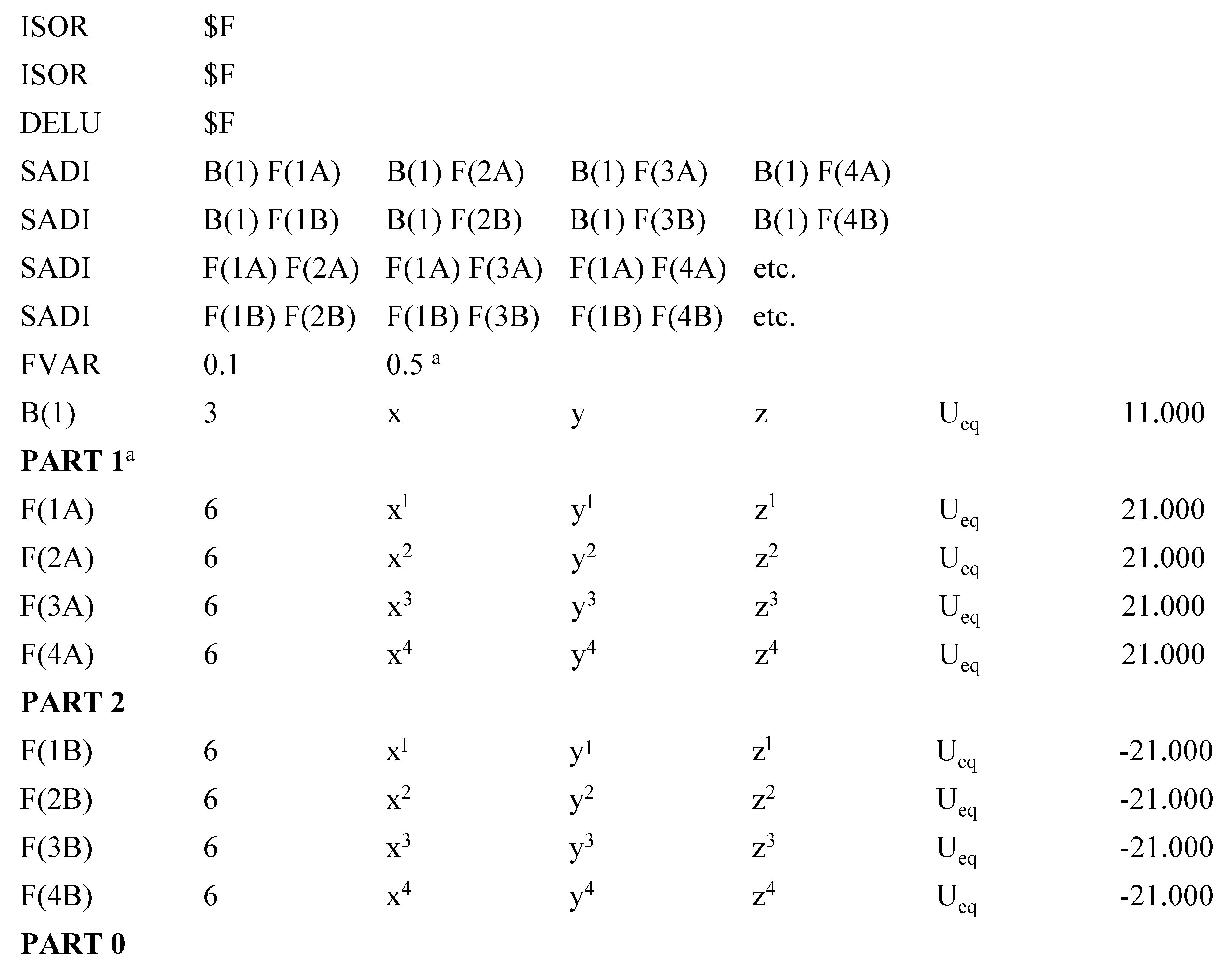
In most cases, this disorder is easily resolved as some non-crystallographic symmetry elements acting locally on the weakly coordinating anion. The atomic site occupancies can be refined using the FVAR instruction on the different parts (see PART 1 and PART 2 in Figure \(\PageIndex{47}\)) of the disorder, having a site occupancy factor (s.o.f.) of x and 1-x, respectively. This is accomplished by replacing 11.000 (on the F-atom lines in the “NAME.INS” file) with 21.000 or -21.000 for each of the different parts of the disorder. For instance, the "NAME.INS" file would look something like that shown in Figure \(\PageIndex{47}\). Note that for more heavily disordered structures, i.e., those with more than two disordered parts, the SUMP command can be used to determine the s.o.f. of parts 2, 3, 4, etc. the combined sum of which is set at s.o.f. = 1.0. These are designated in FVAR as the second, third, and fourth terms.
In small molecule refinement, the case will inevitably arise in which some kind of restraints or constraints must be used to achieve convergence of the data. A restraint is any additional information concerning a given structural feature, i.e., limits on the possible values of parameters, may be added into the refinement, thereby increasing the number of refined parameters. For example, aromatic systems are essentially flat, so for refinement purposes, a troublesome ring system could be restrained to lie in one plane. Restraints are not exact, i.e., they are tied to a probability distribution, whereas constraints are exact mathematical conditions. Restraints can be regarded as falling into one of several general types:
- Geometric restraints, which relates distances that should be similar.
- Rigid group restraints.
- Anti-bumping restraints.
- Linked parameter restraints.
- Similarity restraints.
- ADP restraints (Figure \(\PageIndex{48}\)
- Sum and average restraints.
- Origin fixing and shift limiting restraints.
- Those imposed upon atomic displacement parameters.
Geometric Restraints
- SADI - similar distance restraints for named pairs of atoms.
- DFIX - defined distance restraint between covalently bonded atoms.
- DANG - defined non-bonding distance restraints, e.g., between F atoms belonging to the same PART of a disordered BF4-.
- FLAT - restrains group of atoms to lie in a plane.
Anisotropic Displacement Parameter Restraints
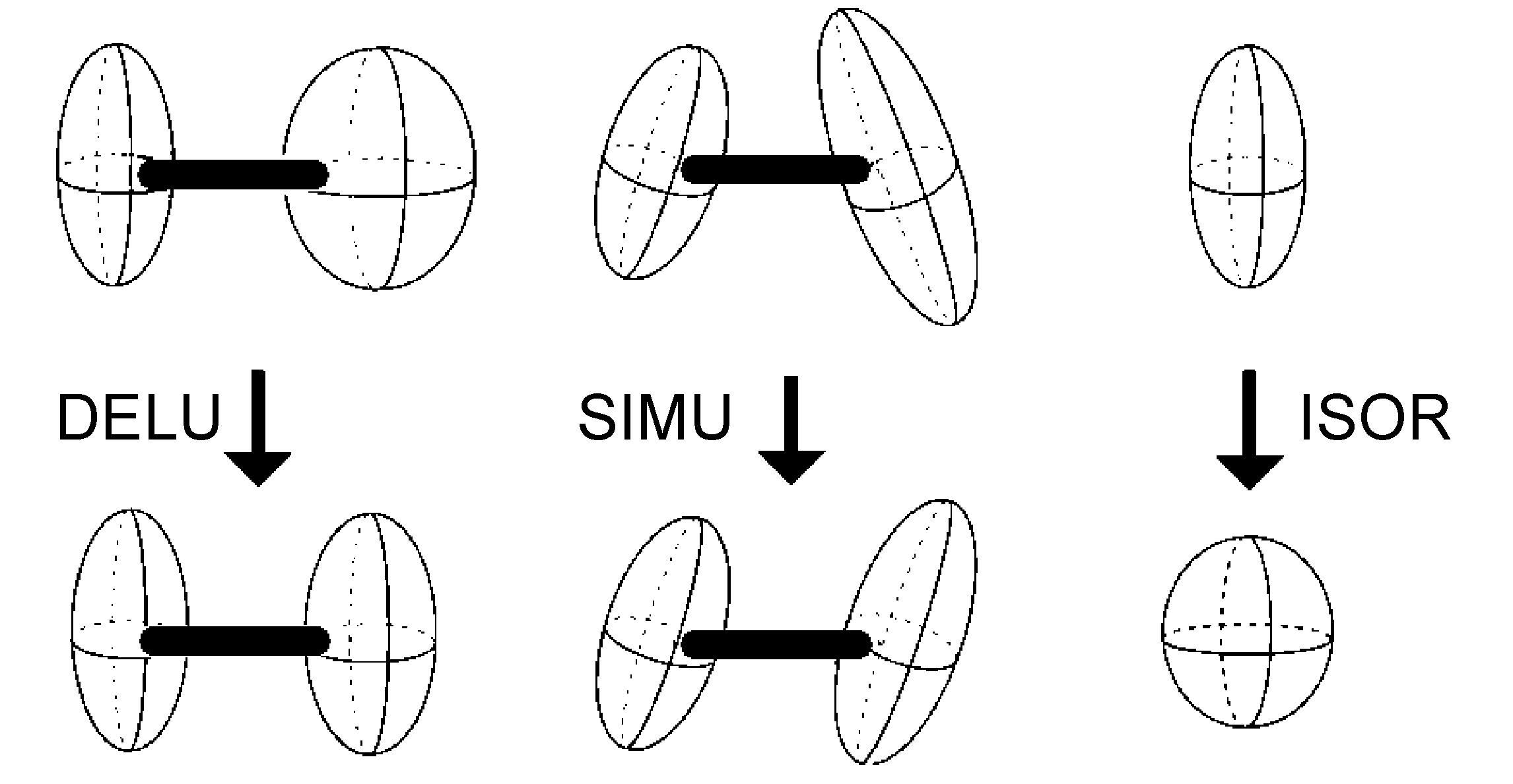
- DELU - rigid bond restraints (Figure \(\PageIndex{48}\))
- SIMU - similar ADP restraints on corresponding Uij components to be approximately equal for atoms in close proximity (Figure \(\PageIndex{48}\))
- ISOR - treat named anisotropic atoms to have approximately isotropic behavior (Figure \(\PageIndex{48}\))
Constraints (different than "restraints")
- EADP - equivalent atomic displacement parameters.
- AFIX - fitted group; e.g., AFIX 66 would fit the next six atoms into a regular hexagon.
- HFIX - places H atoms in geometrically ideal positions, e.g., HFIX 123 would place two sets of methyl H atoms disordered over two sites, 180° from each other.
Classess of Disorder for the Tetrafluoroborate Anion
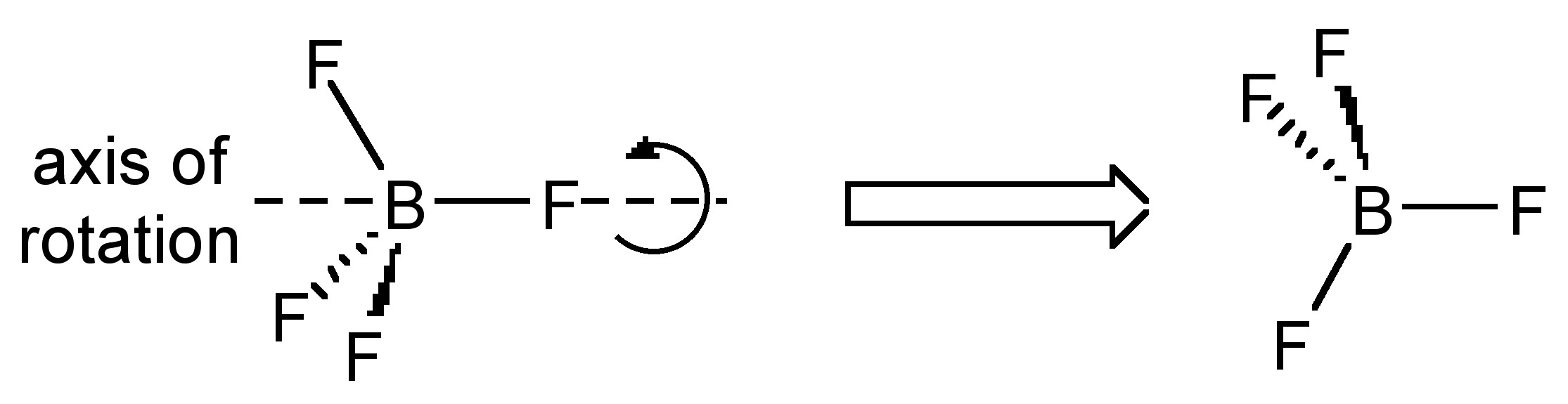
Rotating about a non-crystallographic axis along a B-F bond
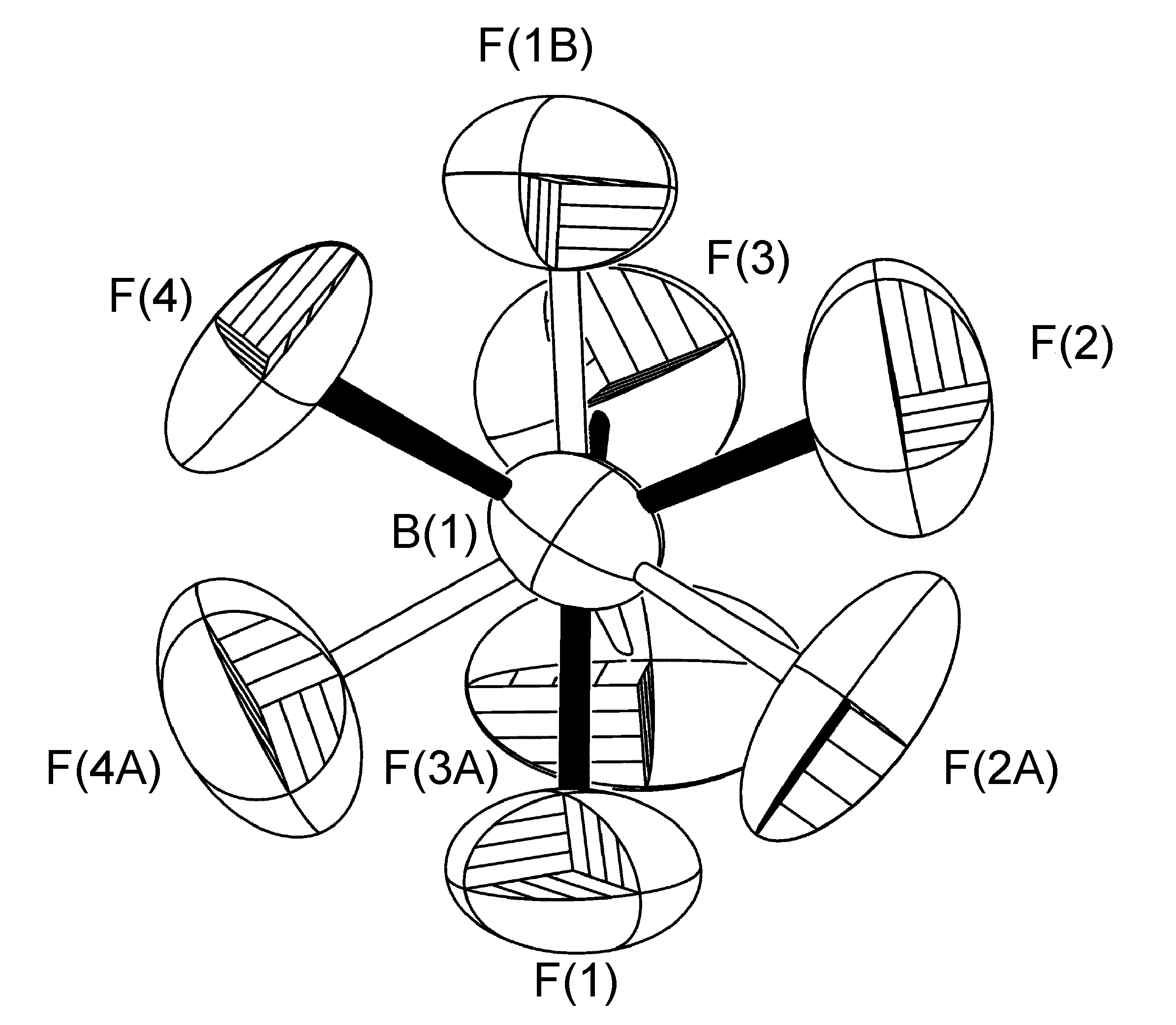
The most common case of disorder is a rotation about an axis, the simplest of which involves a non-crystallographic symmetry related rotation axis about the vector made by one of the B-F bonds; this operation leads to three of the four F-atoms having two site occupancies (Figure \(\PageIndex{49}\)). This disorder is also seen for tBu and CF3 groups, and due to the C3 symmetry of the C(CH3)3, CF3 and BF3 moieties actually results in a near C2rotation.
In a typical example, the BF4- anion present in the crystal structure of [H(Mes-dpa)]BF4 (Figure \(\PageIndex{50}\)) was found to have a 75:25 site occupancy disorder for three of the four fluorine atoms (Figure \(\PageIndex{51}\)). The disorder is a rotation about the axis of the B(1)-F(1) bond. For initial refinement cycles, similar distance restraints (SADI) were placed on all B-F and F-F distances, in addition to similar ADP restraints (SIMU) and rigid bond restraints (DELU) for all F atoms. Restraints were lifted for final refinement cycles. A similar disorder refinement was required for [H(2-iPrPh-dpa)]BF4 (45:55), while refinement of the disorder in [Cu(2-iPrPh-dpa)(styrene)]BF4(65:35) was performed with only SADI and DELU restraints were lifted in final refinement cycles.
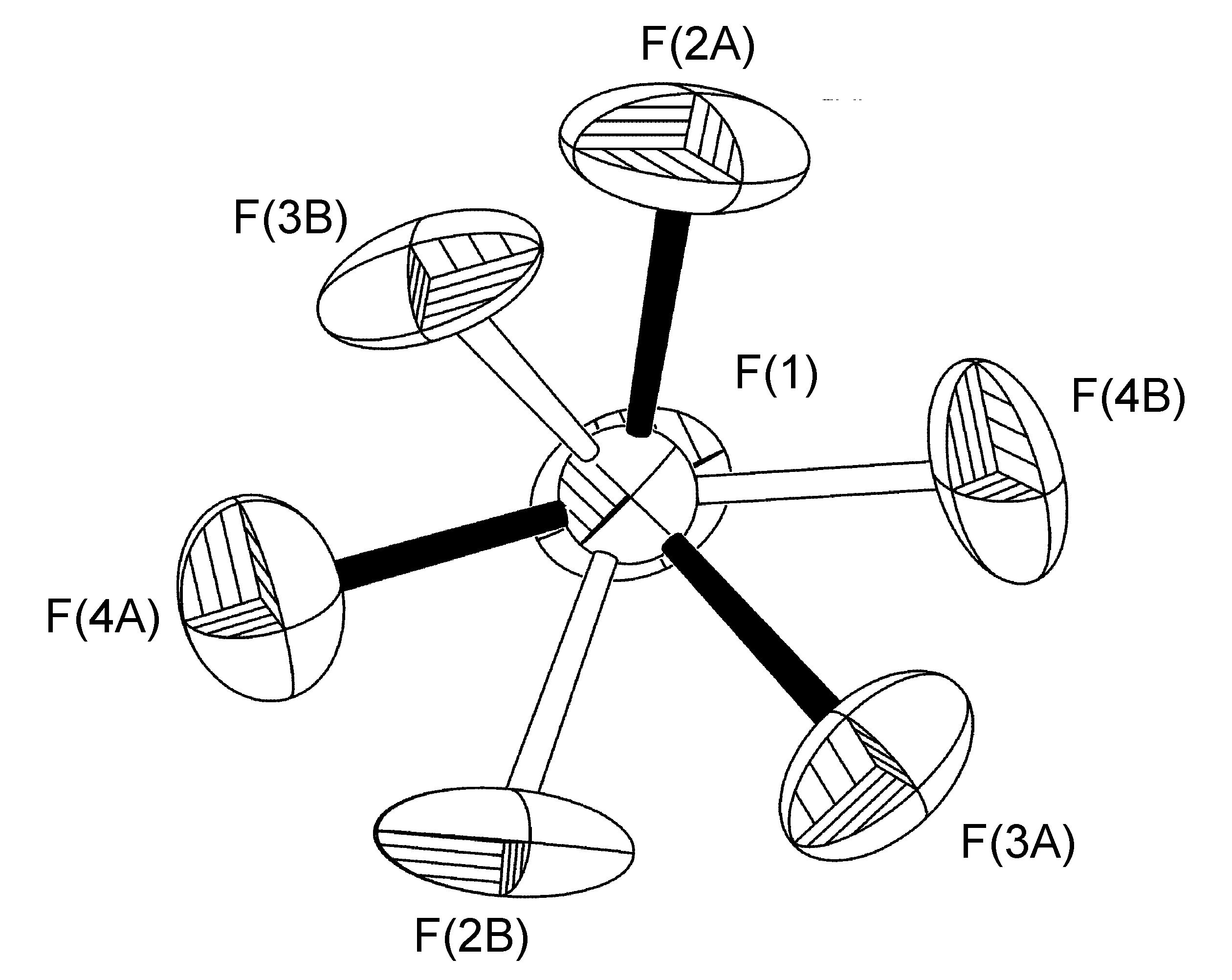
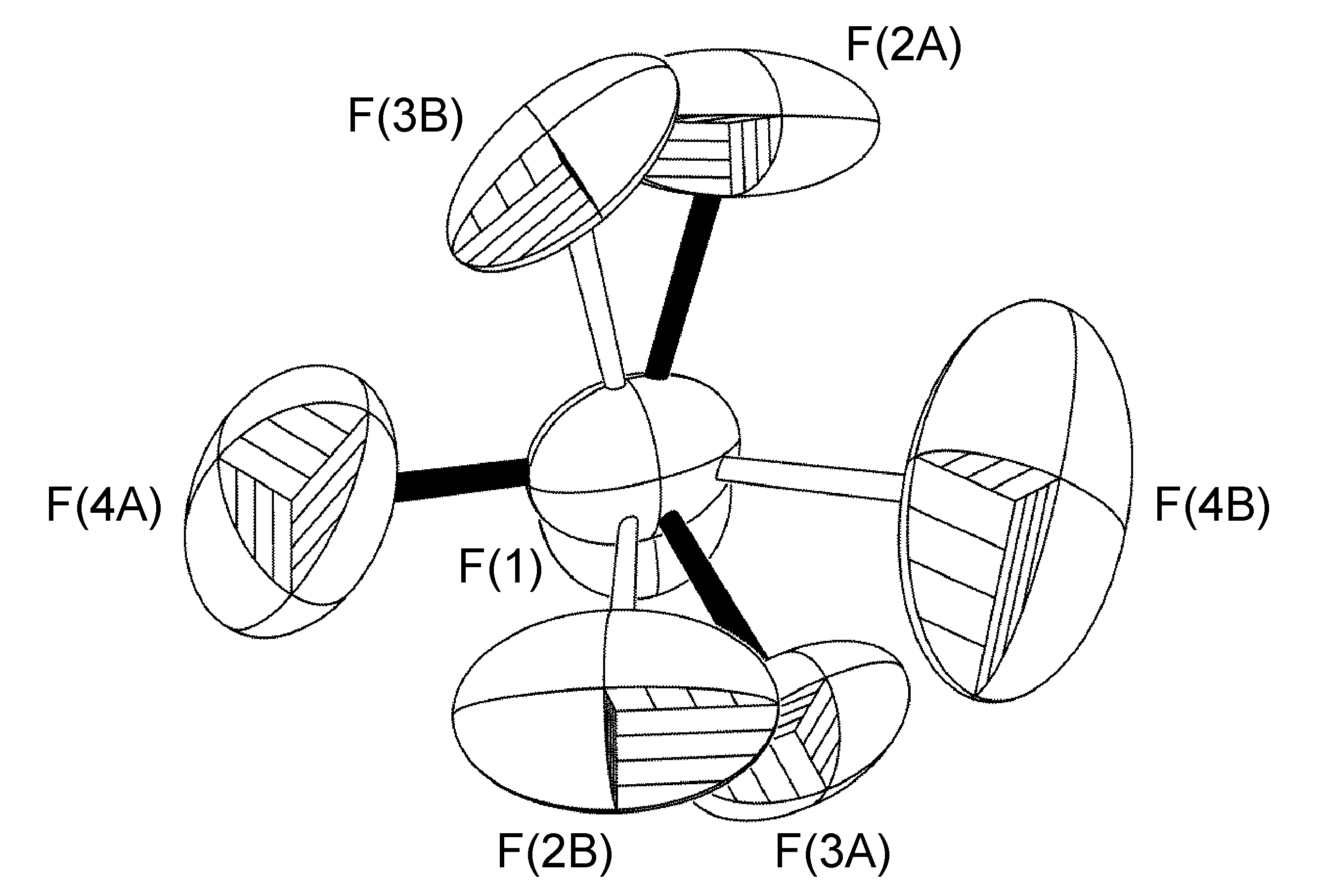
In the complex [Ag(H-dpa)(styrene)]BF4 use of the free variable (FVAR) led to refinement of disordered fluorine atoms F(2A)-F(4A) and F(2B)-F(4B) as having a 75:25 site-occupancy disorder (Figure \(\PageIndex{52}\)). For initial refinement cycles, all B-F bond lengths were given similar distance restraints (SADI). Similar distance restraints (SADI) were also placed on F…F distances for each part, i.e., F(2A)…F(3A) = F(2B)…F(3B), etc. Additionally, similar ADP restraints (SIMU) and rigid bond restraints (DELU) were placed on all F atoms. All restraints, with the exception of SIMU, were lifted for final refinement cycles.
Rotation About a Non-Crystallographic Axis not Along a B-F Bond
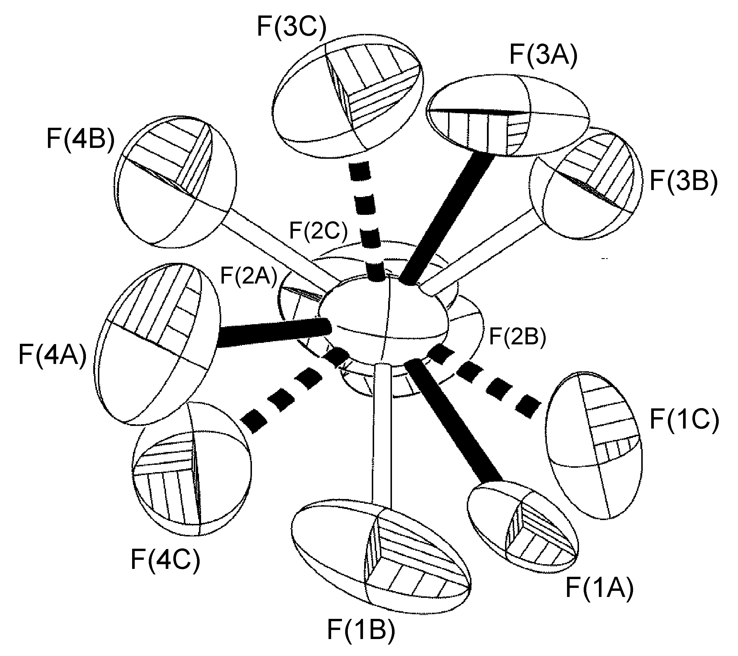
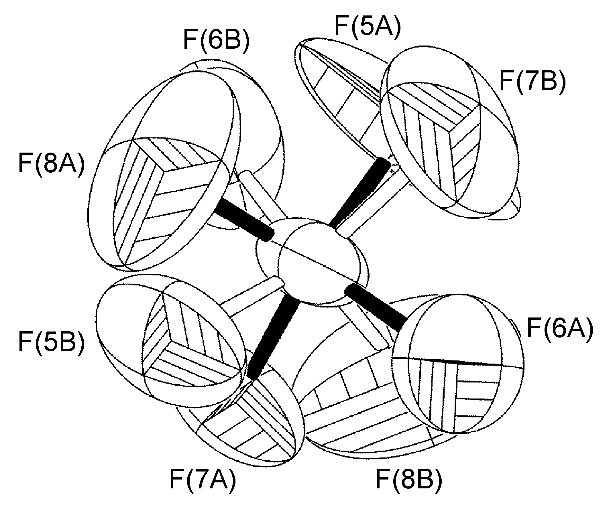
The second type of disorder is closely related to the first, with the only difference being that the rotational axis is tilted slightly off the B-F bond vector, resulting in all four F-atoms having two site occupancies (Figure \(\PageIndex{53}\)). Tilt angles range from 6.5° to 42°.
The disordered BF4- anion present in the crystal structure of [Cu(Ph-dpa)(styrene)]BF4 was refined having fractional site occupancies for all four fluorine atoms about a rotation slightly tilted off the B(1)-F(2A) bond. However, it should be noted that while the U(eq) values determined for the data collected at low temperature data is roughly half that of that found at room temperature, as is evident by the sizes and shapes of fluorine atoms in Figure \(\PageIndex{54}\), the site occupancies were refined to 50:50 in each case, and there was no resolution in the disorder.

An extreme example of rotation off-axis is observed where refinement of more that two site occupancies (Figure \(\PageIndex{55}\)) with as many as thirteen different fluorine atom locations on only one boron atom.
Constrained Rotation About a Non-Crystallographic Axis not Along a B-F Bond
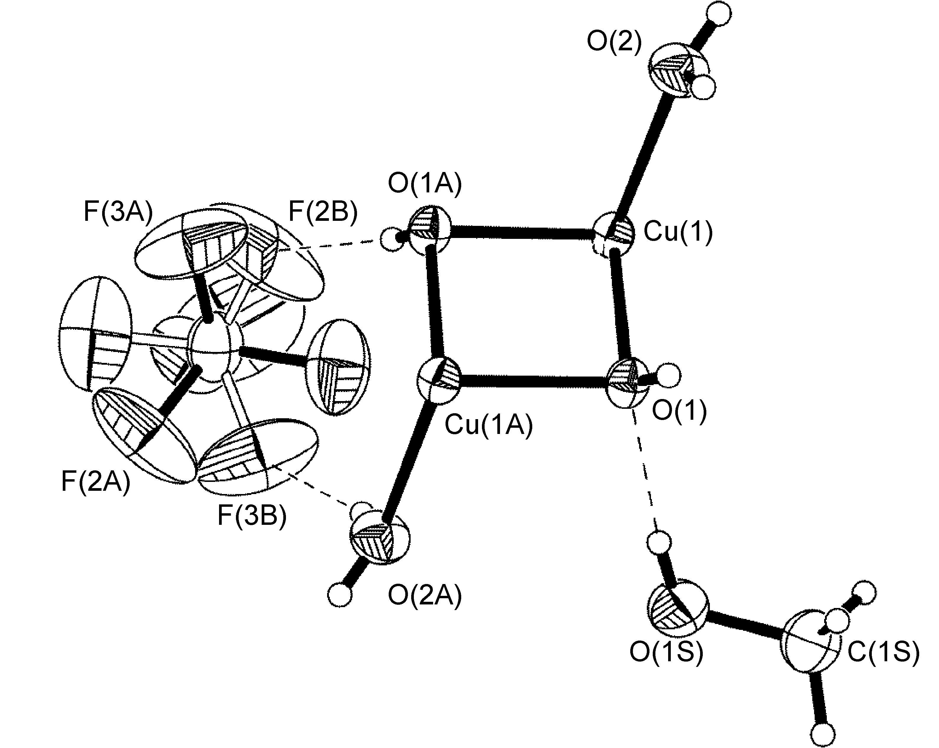
Although a wide range of tilt angles are possible, in some systems the angle is constrained by the presence of hydrogen bonding. For example, the BF4- anion present in [Cu(Mes-dpa)(μ-OH)(H2O)]2[BF4]2 was found to have a 60:40 site occupancy disorder of the four fluorine atoms, and while the disorder is a C2-rotation slightly tilted off the axis of the B(1)-F(1A) bond, the angle is restricted by the presence of two B-F…O interactions for one of the isomers (Figure \(\PageIndex{56}\)).
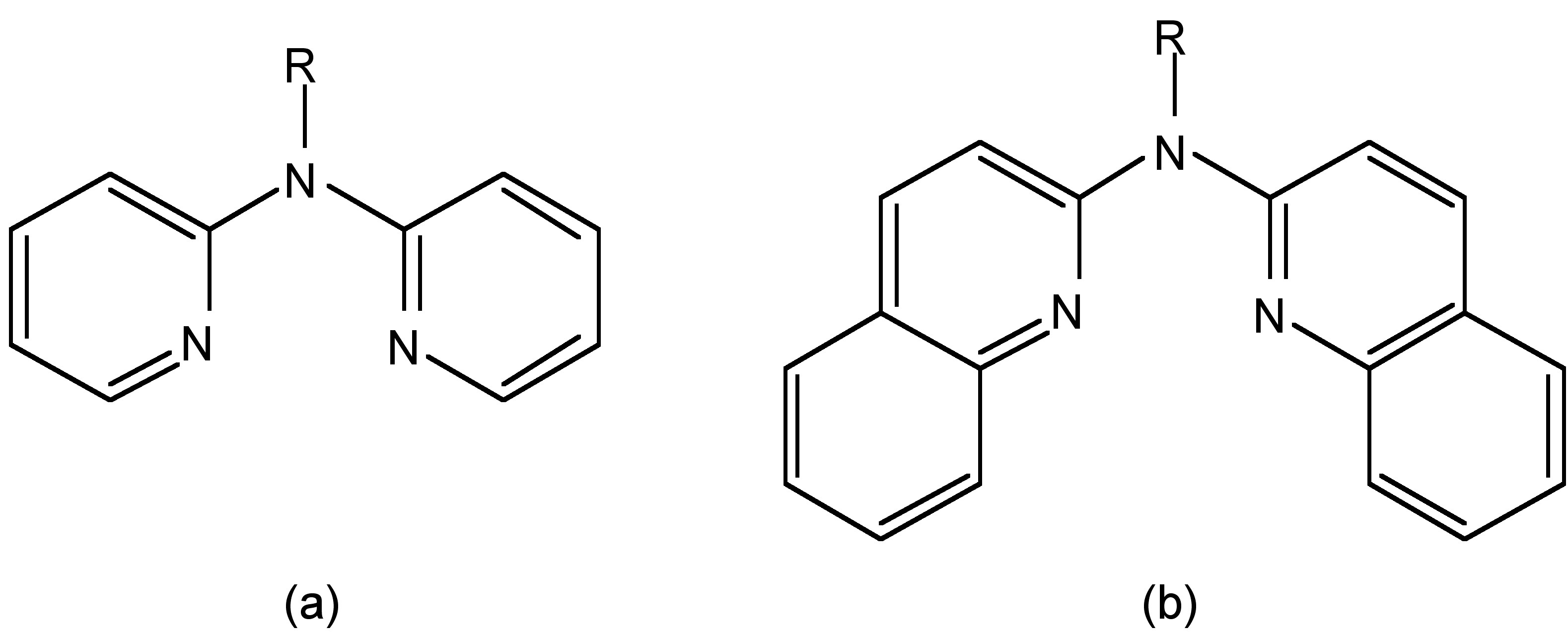
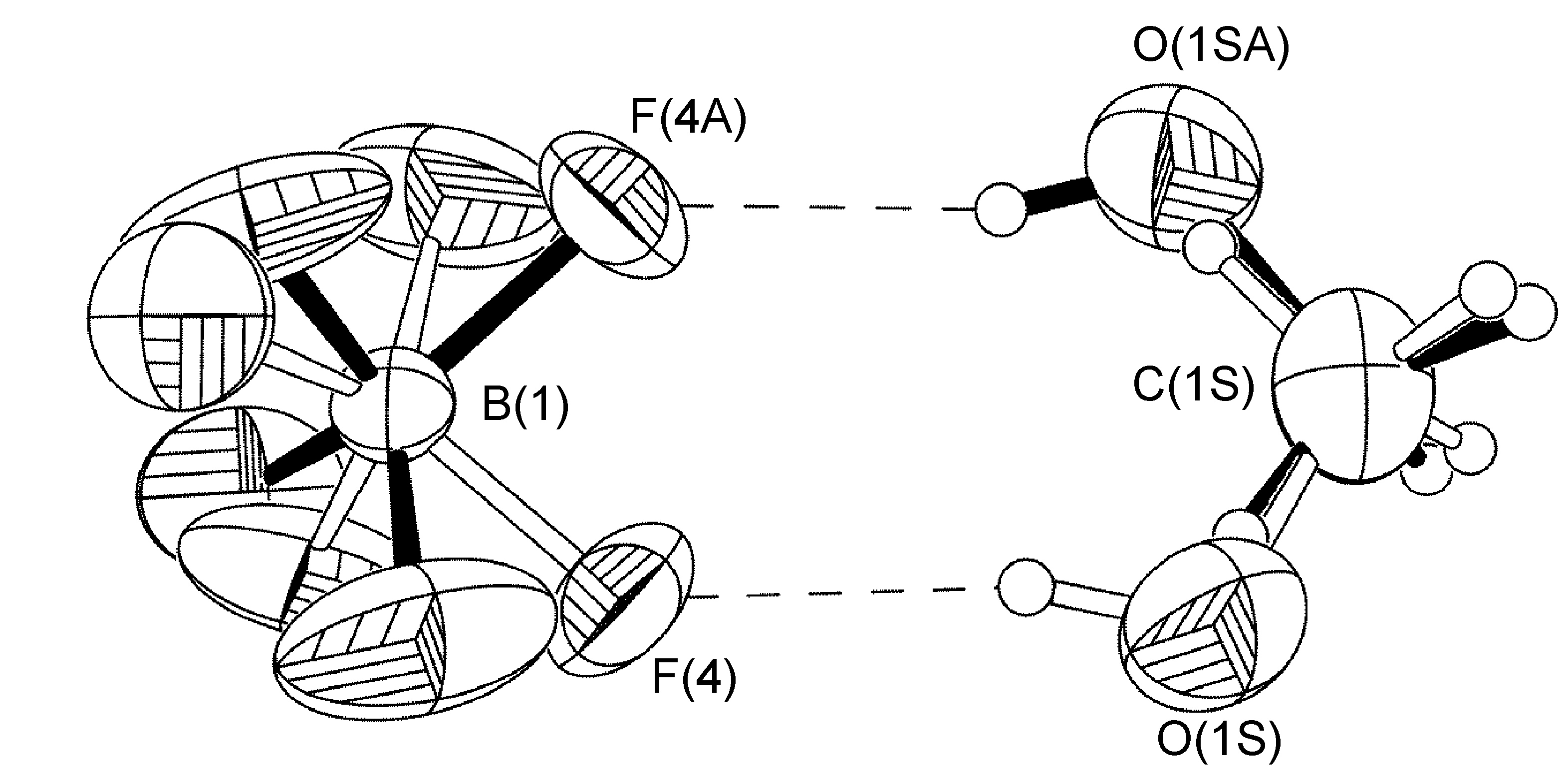
An example that does adhere to global symmetry elements is seen in the BF4- anion of [Cu{2,6-iPr2C6H3N(quin)2}2]BF4.MeOH (Figure \(\PageIndex{57}\)), which exhibits a hydrogen-bonding interaction with a disordered methanol solvent molecule. The structure of R-N(quin)2 is shown in Figure \(\PageIndex{54}\) b. By crystallographic symmetry, the carbon atom from methanol and the boron atom from the BF4- anion lie on a C2-axis. Fluorine atoms [F(1)-F(4)], the methanol oxygen atom, and the hydrogen atoms attached to methanol O(1S) and C(1S) atoms were refined as having 50:50 site occupancy disorder (Figure \(\PageIndex{57}\)).
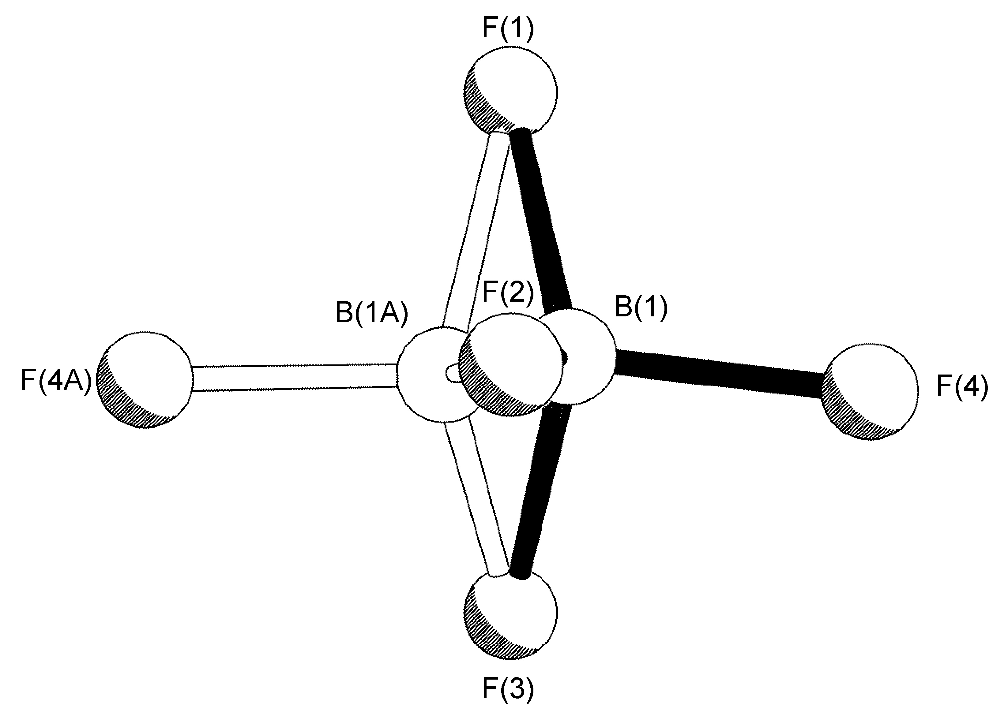
Non Crystallographic Inversion Center at the Boron Atom
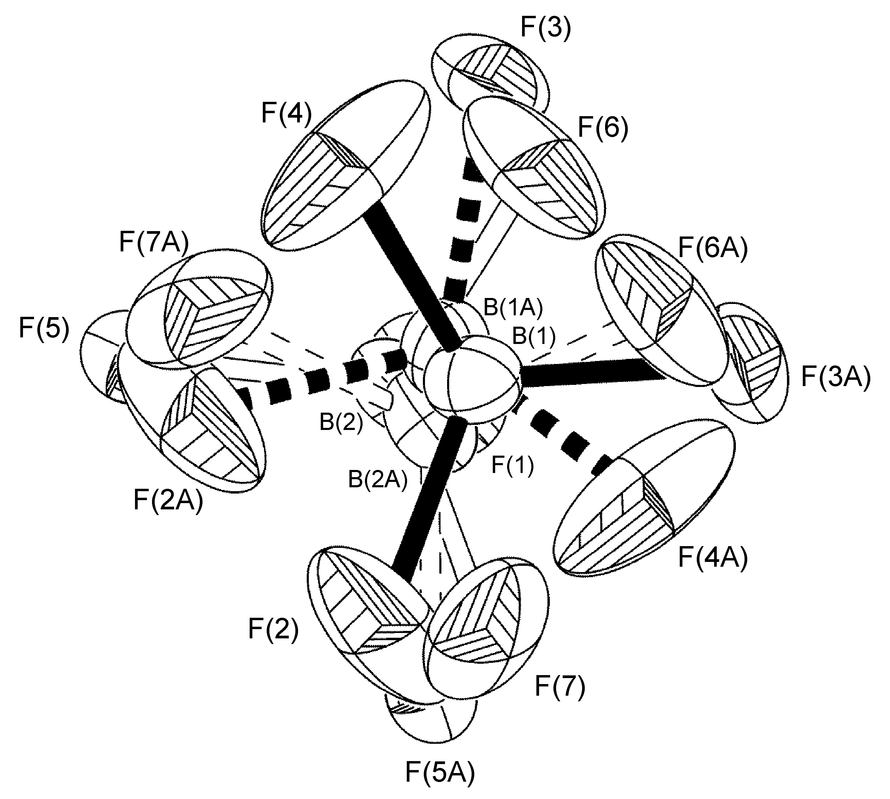
Multiple disorders can be observed with a single crystal unit cell. For example, the two BF4- anions in [Cu(Mes-dpa)(styrene)]BF4 both exhibited 50:50 site occupancy disorders, the first is a C2-rotation tilted off one of the B-F bonds, while the second is disordered about an inversion centered on the boron atom. Refinement of the latter was carried out similarly to the aforementioned cases, with the exception that fixed distance restraints for non-bonded atoms (DANG) were left in place for the disordered fluorine atoms attached to B(2) (Figure \(\PageIndex{58}\)).
Disorder on a Crystallographic Mirror Plane
Another instance in which the BF4- anion is disordered about a crystallographic symmetry element is that of [Cu(H-dpa)(1,5-cyclooctadiene)]BF4. In this instance fluorine atoms F(1) through F(4) are present in the asymmetric unit of the complex. Disordered atoms F(1A)-F(4A) were refined with 50% site occupancies, as B(1) lies on a mirror plane (Figure \(\PageIndex{59}\)). For initial refinement cycles, similar distance restraints (SADI) were placed on all B-F and F-F distances, in addition to similar ADP restraints (SIMU) and rigid bond restraints (DELU) for all F atoms. Restraints were lifted for final refinement cycles, in which the boron atom lies on a crystallographic mirror plane, and all four fluorine atoms are reflected across.

Disorder on a Non-Crystallographic Mirror Plane
It has been observed that the BF4- anion can exhibit site occupancy disorder of the boron atom and one of the fluorine atoms across an NCS mirror plane defined by the plane of the other three fluorine atoms (Figure \(\PageIndex{60}\)) modeling the entire anion as disordered (including the boron atom).
Disorder of the Boron Atom Core
The extreme case of a disorder involves refinement of the entire anion, with all boron and all fluorine atoms occupying more than two sites (Figure \(\PageIndex{61}\)). In fact, some disorders of the latter types must be refined isotropically, or as a last-resort, not at all, to prevent one or more atoms from turning non-positive definite.