
6.2: Determination of Energetics of Fluxional Molecules by NMR
- Page ID
- 55901

Introduction to Fluxionality
It does not take an extensive knowledge of chemistry to understand that as-drawn chemical structures do not give an entirely correct picture of molecules. Unlike drawings, molecules are not stationary objects in solution, the gas phase, or even in the solid state. Bonds can rotate, bend, and stretch, and the molecule can even undergo conformational changes. Rotation, bending, and stretching do not typically interfere with characterization techniques, but conformational changes occasionally complicate analyses, especially nuclear magnetic resonance (NMR).
For the present discussion, a fluxional molecule can be defined as one that undergoes an intramolecular reversible interchange between two or more conformations. Fluxionality is specified as intramolecular to differentiate from ligand exchange and complexation mechanisms, intermolecular processes. An irreversible interchange is more of a chemical reaction than a form of fluxionality. Most of the following examples alternate between two conformations, but more complex fluxionality is possible. Additionally, this module will focus on inorganic compounds. In this module, examples of fluxional molecules, NMR procedures, calculations of energetics of fluxional molecules, and the limitations of the approach will be covered.
Examples of Fluxionality
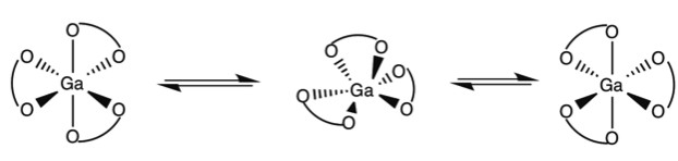
Bailar Twist
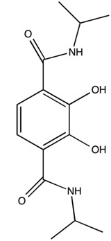
Octahedral trischelate complexes are susceptible to Bailar twists, in which the complex distorts into a trigonal prismatic intermediate before reverting to its original octahedral geometry. If the chelates are not symmetric, a Δ enantiomer will be inverted to a Λ enantiomer. For example not how in Figure \(\PageIndex{1}\) with the GaL3 complex of 2,3-dihydroxy-N,N‘-diisopropylterephthalamide (Figure \(\PageIndex{2}\) he end product has the chelate ligands spiraling the opposite direction around the metal center.
Berry Psuedorotation
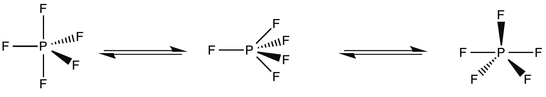
D3h compounds can also experience fluxionality in the form of a Berry pseudorotation (depicted in Figure \(\PageIndex{3}\)), in which the complex distorts into a C4v intermediate and returns to trigonal bipyrimidal geometry, exchanging two equatorial and axial groups . Phosphorous pentafluoride is one of the simplest examples of this effect. In its 19FNMR, only one peak representing five fluorines is present at 266 ppm, even at low temperatures. This is due to interconversion faster than the NMR timescale.
Sandwhich and Half-sandwhich Complexes
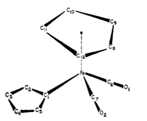
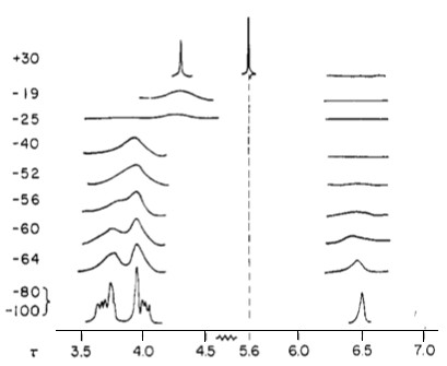
Perhaps one of the best examples of fluxional metal complexes is (π5-C5H5)Fe(CO)2(π1-C5H5) (Figure \(\PageIndex{4}\). Not only does it have a rotating η5 cyclopentadienyl ring, it also has an alternating η1 cyclopentadienyl ring (Cp). This can be seen in its NMR spectra in Figure \(\PageIndex{5}\). The signal for five protons corresponds to the metallocene Cp ring (5.6 ppm). Notice how the peak remains a sharp singlet despite the large temperature sampling range of the spectra. Another noteworthy aspect is how the multiplets corresponding to the other Cp ring broaden and eventually condense into one sharp singlet.
An Example Procedure
ample preparation is essentially the same for routine NMR. The compound of interest will need to be dissolved in an NMR compatible solvent (CDCl3 is a common example) and transferred into an NMR tube. Approximately 600 μL of solution is needed with only micrograms of compound. Compounds should be at least 99 % pure in order to ease peak assignments and analysis. Because each spectrometer has its own protocol for shimming and optimization, having the supervision of a trained specialist is strongly advised. Additionally, using an NMR with temperature control is essential. The basic goal of this experiment is to find three temperatures: slow interchange, fast interchange, and coalescence. Thus many spectra will be needed to be obtained at different temperatures in order to determine the energetics of the fluctuation.
The process will be much swifter if the lower temperature range (in which the fluctuation is much slower than the spectrometer timescale) is known. A spectra should be taken in this range. Spectra at higher temperatures should be taken, preferably in regular increments (for instance, 10 K), until the peaks of interest condense into a sharp single at higher temperature. A spectrum at the coalescence temperature should also be taken in case of publishing a manuscript. This procedure should then be repeated in reverse; that is, spectra should be taken from high temperature to low temperature. This ensures that no thermal reaction has taken place and that no hysteresis is observed. With the data (spectra) in hand, the energetics can now be determined.
Calculation of Energetics
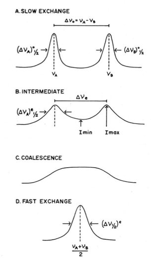
For intramolecular processes that exchange two chemically equivalent nuclei, the function of the difference in their resonance frequencies (Δv) and rate of exchange (k) is the NMR spectrum. Slow interchange occurs when Δv >> k, and two separate peaks are observed. When Δv << k, fast interchange is said to occur, and one sharp peak is observed. At intermediate temperatures, the peaks are broadened and overlap one another. When they completely merge into one peak, the coalescence temperature, Tc is said to be reached. In the case of coalescence of an equal doublet (for instance, one proton exchanging with one proton), coalescences occurs when Δv0t = 1.4142/(2π), where Δv0 is the difference in chemical shift at low interchange and where t is defined by \ref{1}, where ta and tb are the respective lifetimes of species a and b. This condition only occurs when ta = tb, and as a result, k = ½ t.
\[ \frac{1}{t} \ =\ \frac{1}{t_{a}}\ +\ \frac{1}{t_{b}} \label{1} \]
For reference, the exact lineshape function (assuming two equivalent groups being exchanged) is given by the Bloch Equation, \ref{2}, where g is the intensity at frequency v,and where K is a normalization constant.
\[ g(v)= \frac{Kt(v_{a} + v_{b})^{2}}{[0.5(v_{a} + v_{b})- u ]^{2}+4\pi^{2}t^{2}(v_{a}-v)^{2}(v _{b} - v)^{2}} \label{2} \]
Low Temperatures to Coalescence Temperature
At low temperature (slow exchange), the spectrum has two peaks and Δv >> t. As a result, \ref{3} reduces to \ref{4}, where T2a is the spin-spin relaxation time. The linewidth of the peak for species a is defined by \ref{5}.
\[ g(v)_{a}=g(v)_{b}=\frac{KT_{2a}}{1+T^{2}_{2a}(v_{a}-v)^{2}} \label{3} \]
\[ (\Delta v_{a})_{1/2} = \frac{1}{\pi}(\frac{1}{T_{2a}}+\frac{1}{t_{a}} ) \label{4} \]
Because the spin-spin relaxation time is difficult to determine, especially in inhomogeneous environments, rate constants at higher temperatures but before coalescence are preferable and more reliable.
The rate constant k can then be determined by comparing the linewidth of a peak with no exchange (low temp) with the linewidth of the peak with little exchange using, \ref{5}, where subscript e refers to the peak in the slightly higher temperature spectrum and subscript 0 refers to the peak in the no exchange spectrum.
\[ k = \frac{\pi }{ \sqrt{2}}[(\Delta v_{e})_{1/2}- (\Delta v_{0})_{1/2}] \label{5} \]
Additionally, k can be determined from the difference in frequency (chemical shift) using \ref{6}, where Δv0is the chemical shift difference in Hz at the no exchange temperature and Δve is the chemical shift difference at the exchange temperature.
\[ k= \frac{\pi}{\sqrt{2} }(\Delta v^{2}_{0} - \Delta v^{2}_{e}) \label{6} \]
The intensity ratio method, \ref{7}, can be used to determine the rate constant for spectra whose peaks have begun to merge, where r is the ratio between the maximum intensity and the minimum intensity, of the merging peaks, Imax/Imin.
\[ k = \frac{\pi }{\sqrt{2}} (r+(r^{2} - r)^{1/2})^{-1/2} \label{7} \]
Additionally, k can be determined from the difference in frequency (chemical shift) using \ref{8}, where Δv0is the chemical shift difference in Hz at the no exchange temperature and Δve is the chemical shift difference at the exchange temperature.
\[ k\ = \frac{\pi }{\sqrt{2} }(\Delta v^{2}_{0} - \Delta v^{2}_{e} ) \label{8} \]
The intensity ratio method, \ref{9} can be used to determine the rate constant for spectra whose peaks have begun to merge, where r is the ratio between the maximum intensity and the minimum intensity, of the merging peaks, Imax/Imin
\[ k\ = \frac{\pi }{\sqrt{2} }(r+(r^{2}-r)^{1/2})^{-1/2} \label{9} \]
As mentioned earlier, the coalescence temperature, Tc is the temperature at which the two peaks corresponding to the interchanging groups merge into one broad peak and \ref{10} may be used to calculate the rate at coalescence.
\[ k\ = \frac{\pi \Delta v_{0} }{\sqrt{2}} \label{10} \]
Higher Temperatures
Beyond the coalescence temperature, interchange is so rapid (k >> t) that the spectrometer registers the two groups as equivalent and as one peak. At temperatures greater than that of coalescence, the lineshape equation reduces to \ref{11}.
\[ g(v)\ = \frac{KT_{2}}{[1 \ +\ \pi T_{2}(v_{a} \ +\ v_{b} \ +\ 2v)^{2}]} \label{11} \]
As mentioned earlier, determination of T2 is very time consuming and often unreliable due to inhomogeneity of the sample and of the magnetic field. The following approximation (\ref{12}) applies to spectra whose signal has not completely fallen (in their coalescence).
\[ k\ = \frac{ 0.5\pi \Delta v^{2} }{(\Delta v_{e})_{1/2} - (\Delta v_{0} )_{1/2} } \label{12} \]
Now that the rate constants have been extracted from the spectra, energetic parameters may now be calculated. For a rough measure of the activation parameters, only the spectra at no exchange and coalescence are needed. The coalescence temperature is determined from the NMR experiment, and the rate of exchange at coalescence is given by \ref{10}. The activation parameters can then be determined from the Eyring equation (\ref{13} ), where kB is the Boltzmann constant, and where ΔH‡ - TΔS‡ = ΔG‡.
\[ ln(\frac{k}{t}) = \frac{\Delta H^{\ddagger } }{RT} - \frac{\Delta S^{\ddagger }}{R} + ln(\frac{k_{B}}{h}) \label{13} \]
For more accurate calculations of the energetics, the rates at different temperatures need to be obtained. A plot of ln(k/T) versus 1/T (where T is the temperature at which the spectrum was taken) will yield ΔH‡, ΔS‡, and ΔG‡. For a pictorial representation of these concepts, see Figure \(\PageIndex{6}\).
Diverse Populations
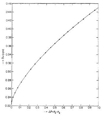
For unequal doublets (for instance, two protons exchanging with one proton), a different treatment is needed. The difference in population can be defined through \ref{14}, where Pi is the concentration (integration) of species i and X = 2πΔvt (counts per second). Values for Δvt are given in Figure \(\PageIndex{7}\).
\[ \Delta P = P_{a} - P_{b} = [ \frac{X^{2} - 2}{3} ]^{3/2} (\frac{1}{X}) \label{14} \]
The rates of conversion for the two species, ka and kb, follow kaPa = kbPb (equilibrium), and because ka = 1/taand kb = 1/tb, the rate constant follows \ref{15}.
\[ k_{i} = \frac{1}{2t}(1- \Delta P) \label{15} \]
From Erying's expressions, the Gibbs free activation energy for each species can be obtained through \ref{16} and \ref{17}.
\[ \Delta G^{\ddagger }_{a} = \ RT_{c}\ ln(\frac{kT_{c}}{h\pi \Delta v_{0}} \times \frac{X}{1-\Delta P_{a}} ) \label{16} \]
\[ \Delta G^{\ddagger }_{b} = \ RT_{c}\ ln(\frac{kT_{c}}{h\pi \Delta v_{0}} \times \frac{X}{1-\Delta P_{b}} ) \label{17} \]
Taking the difference of \ref{16} and \ref{17} gives the difference in energy between species a and b (\ref{18}).
\[ \Delta G^{\ddagger } = RT_{c} ln(\frac{P_{a}}{P_{b}}=RT_{c}ln(\frac{1+P}{1-P}) \label{18} \]
Converting constants will yield the following activation energies in calories per mole (\ref{19} and \ref{20}).
\[ \Delta G^{\ddagger }_{a} = 4.57T_{c}[10.62\ +\ log(\frac{X}{2p(1-\Delta P)}) +\ log(T_{c}/\Delta v)] \label{19} \]
\[ \Delta G^{\ddagger }_{b} = 4.57T_{c}[10.62\ +\ log(\frac{X}{2p(1-\Delta P)}) +\ log(T_{c}/\Delta v)] \label{20} \]
To obtain the free energys of activation, values of log (X/(2π(1 + ΔP))) need to be plotted against ΔP (values Tc and Δv0 are predetermined).
This unequal doublet energetics approximation only gives ΔG‡ at one temperature, and a more rigorous theoretical treatment is needed to give information about ΔS‡ and ΔH‡.
Example of Determination of Energetic Parameters
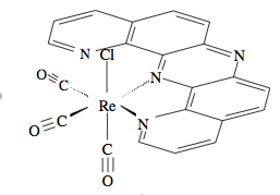
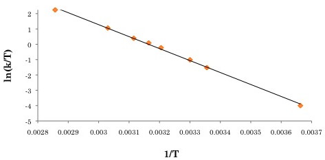
Normally ligands such as dipyrido(2,3-a;3′,2′-j)phenazine (dpop’) are tridentate when complexed to transition metal centers. However, dpop’ binds to rhenium in a bidentate manner, with the outer nitrogens alternating in being coordinated and uncoordinated. See Figure \(\PageIndex{8}\)for the structure of Re(CO)3(dpop')Cl. This fluxionality results in the exchange of the aromatic protons on the dpop’ ligand, which can be observed via 1HNMR. Because of the complex nature of the coalescence of doublets, the rate constants at different temperatures were determined via computer simulation (DNMR3, a plugin of Topspin). These spectra are shown in Figure \(\PageIndex{8}\).

The activation parameters can then be obtained by plotting ln(k/T) versus 1/T (see Figure \(\PageIndex{9}\) for the Eyring plot). ΔS‡ can be extracted from the y-intercept, and ΔH‡ can be obtained through the slope of the plot. For this example, ΔH‡, ΔS‡ and ΔG‡. were determined to be 64.9 kJ/mol, 7.88 J/mol, and 62.4 kJ/mol.
Limitations to the Approach
Though NMR is a powerful technique for determining the energetics of fluxional molecules, it does have one major limitation. If the fluctuation is too rapid for the NMR timescale (< 1 ms) or if the conformational change is too slow meaning the coalescence temperature is not observed, the energetics cannot be calculated. In other words, spectra at coalescence and at no exchange need to be observable. One is also limited by the capabilities of the available spectrometer. The energetics of very fast fluxionality (metallocenes, PF5, etc) and very slow fluxionality may not be determinable. Also note that this method does not prove any fluxionality or any mechanism thereof; it only gives a value for the activation energy of the process. As a side note, sometimes the coalescence of NMR peaks is not due to fluxionality, but rather temperature-dependent chemical shifts.