2.9: Electrical Permittivity Characterization of Aqueous Solutions
- Page ID
- 55855

Introduction
Permittivity (in the framework of electromagnetics) is a fundamental material property that describes how a material will affect, and be affected by, a time-varying electromagnetic field. The parameters of permittivity are often treated as a complex function of the applied electromagnetic field as complex numbers allow for the expression of magnitude and phase. The fundamental equation for the complex permittivity of a substance (εs) is given by \ref{1} , where ε’ and ε’’ are the real and imaginary components, respectively, ω is the radial frequency (rad/s) and can be easily converted to frequency (Hertz, Hz) using \ref{2} .
\[ \varepsilon _{s} = \varepsilon ' ( \omega )\ -\ i\varepsilon ''(\omega ) \label{1} \]
\[ \omega \ =\ 2\pi f \label{2} \]
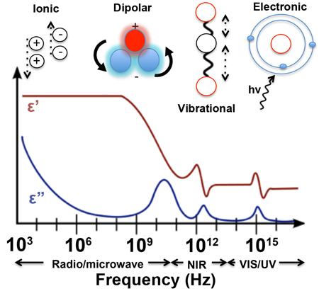
Specifically, the real and imaginary parameters defined within the complex permittivity equation describe how a material will store electromagnetic energy and dissipate that energy as heat. The processes that influence the response of a material to a time-varying electromagnetic field are frequency dependent and are generally classified as either ionic, dipolar, vibrational, or electronic in nature. These processes are highlighted as a function of frequency in Figure \(\PageIndex{1}\). Ionic processes refer to the general case of a charged ion moving back and forth in response a time-varying electric field, whilst dipolar processes correspond to the ‘flipping’ and ‘twisting’ of molecules, which have a permanent electric dipole moment such as that seen with a water molecule in a microwave oven. Examples of vibrational processes include molecular vibrations (e.g. symmetric and asymmetric) and associated vibrational-rotation states that are Infrared (IR) active. Electronic processes include optical and ultra-violet (UV) absorption and scattering phenomenon seen across the UV-visible range.
The most common relationship scientists that have with permittivity is through the concept of relative permittivity: the permittivity of a material relative to vacuum permittivity. Also known as the dielectric constant, the relative permittivity (εr) is given by \ref{3} , where εs is the permittivity of the substance and ε0 is the permittivity of a vacuum (ε0 = 8.85 x 10⁻¹² Farads/m). Although relative permittivity is in fact dynamic and a function of frequency, the dielectric constants are most often expressed for low frequency electric fields where the electric field is essential static in nature. Table \(\PageIndex{1}\) depicts the dielectric constants for a range of materials.
\[ \varepsilon _{r} \ =\ \varepsilon_{s} / \varepsilon_{0} \label{3} \]
| Material | Relative Permittivity |
|---|---|
| Vacuum | 1 (by definition) |
| Air | 1.00058986 |
| Polytetrafluoroethylene (PTFE, Teflon) | 2.1 |
| Paper | 3.85 |
| Diamond | 5.5-10 |
| Methanol | 30 |
| Water | 80.1 |
| Titanium dioxide (TiO2) | 86-173 |
| Strontium titanate (SrTiO3) | 310 |
| Barium titanate (BaTiO3) | 1,200 - 10,000 |
| Calcium copper titanate (CaCu3Ti4O12) | >250,000 |
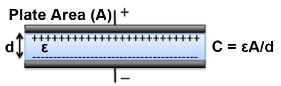
Dielectric constants may be useful for generic applications whereby the high-frequency response can be neglected, although applications such as radio communications, microwave design, and optical system design call for a more rigorous and comprehensive analysis. This is especially true for electrical devices such as capacitors, which are circuit elements that store and discharge electrical charge in both a static and time-varying manner. Capacitors can be thought of as two parallel plate electrodes that are separated by a finite distance and ‘sandwich’ together a piece of material with characteristic permittivity values. As can be seen in Figure \(\PageIndex{2}\), the capacitance is a function of the permittivity of the material between the plates, which in turn is dependent on frequency. Hence, for capacitors incorporated into the circuit design for radio communication applications, across the spectrum 8.3 kHz – 300 GHz, the frequency response would be important as this will determine the capacitors ability to charge and discharge as well as the thermal response from electric fields dissipating their power as heat through the material.
Evaluating the electrical characteristics of materials is become increasingly popular – especially in the field of electronics whereby miniaturization technologies often require the use of materials with high dielectric constants. The composition and chemical variations of materials such as solids and liquids can adopt characteristic responses, which are directly proportional to the amounts and types of chemical species added to the material. The examples given herein are related to aqueous suspensions whereby the electrical permittivity can be easily modulated via the addition of sodium chloride (NaCl).
Instrumentation
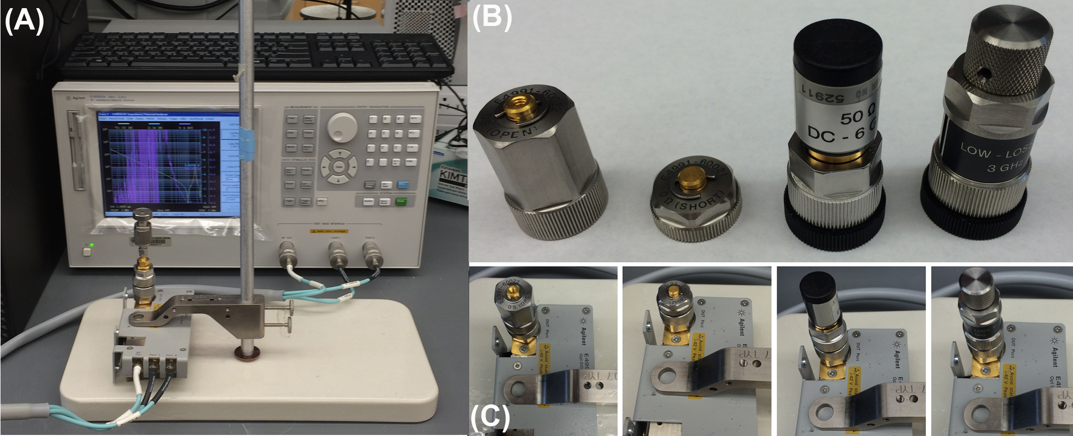
A common and reliable method for measuring the dielectric properties of liquid samples is to use an impedance analyzer in conjunction with a dielectric probe. The impedance analyzer directly measures the complex impedance of the sample under test and is then converted to permittivity using the system software. There are many methods used for measuring impedance, each of which has their own inherent advantages and disadvantages and factors associated with that particular method. Such factors include frequency range, measurement accuracy, and ease of operation. Common impedance measurements include bridge method, resonant method, current-voltage (I-V) method, network analysis method, auto-balancing bridge method, and radiofrequency (RF) I-V method. The RF I-V method used herein has several advantages over previously mentioned methods such as extended frequency coverage, better accuracy, and a wider measured impedance range. The principle of the RF I-V method is based on the linear relationship of the voltage-current ratio to impedance, as given by Ohm’s law (V=IZ where V is voltage, I is current, and Z is impedance). This results in the impedance measurement sensitivity being constant regardless of measured impedance. Although a full description of this method involves circuit theory and is outside the scope of this module (see “Impedance Measurement Handbook” for full details) a brief schematic overview of the measurement principles is shown in Figure \(\PageIndex{3}\).
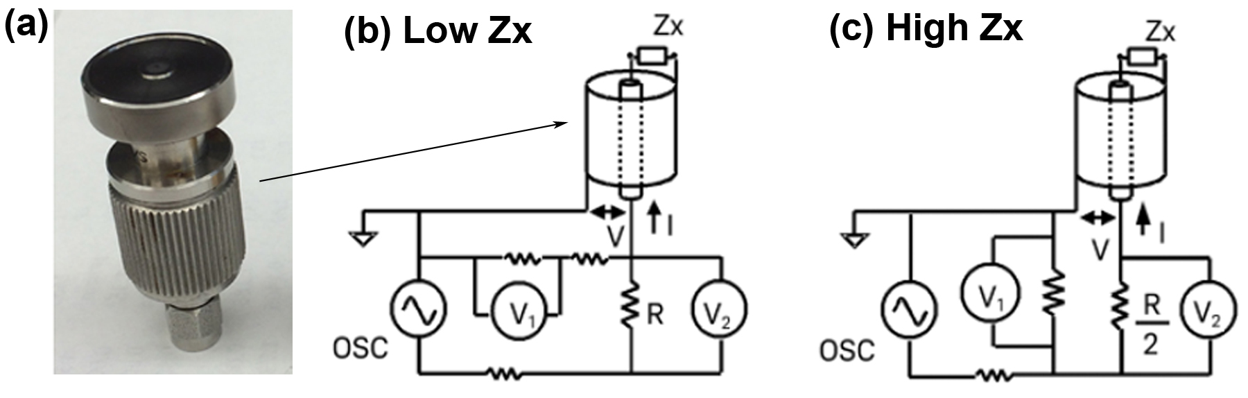
As can be seen in Figure 3, the RF I-V method, which incorporates the use of a dielectric probe, essentially measures variations in voltage and current when a sample is placed on the dielectric probe. For the low-impedance case, the impedance of the sample (Zx) is given by \ref{4} , for a high-impedance sample, the impedance of the sample (Zx) is given by \ref{5} .
\[ Z_{x} \ =\ V/I \ =\frac{2R}{ \frac{V_{2}}{V_{1}}\ -\ 1} \label{4} \]
\[ Z_{x} \ =\ V/I \ =\frac{R}{2}[\frac{V_{1}}{V_{2}} -\ 1] \label{5} \]
The instrumentation and methods described herein consist of an Agilent E4991A impedance analyzer connected to an Agilent 85070E dielectric probe kit. The impedance analyzer directly measures the complex impedance of the sample under test by measuring either the frequency-dependent voltage or current across the sample. These values are then converted to permittivity values using the system software.
Applications
Electrical permittivity of deionized water and saline (0.9 % w/v NaCl)
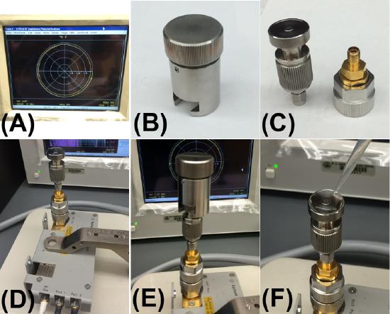
In order to acquire the electrical permittivity of aqueous solutions the impedance analyzer and dielectric probe must first be calibrated. In the first instance, the impedance analyzer unit is calibrated under open-circuit, short-circuit, 50 ohm load, and low loss capacitance conditions by attaching the relevant probes shown in Figure \(\PageIndex{4}\). The dielectric probe is then attached to the system and re-calibrated in open-air, with an attached short circuit probe, and finally with 500 μl of highly purified deionized water (with a resistivity of 18.2 MΩ/cm at 25 °C) (Figure \(\PageIndex{5}\) ). The water is then removed and the system is ready for acquiring data.
In order to maintain accurate calibration only the purest deionized water with a resistivity of 18.2 MΩ/cm at 25 °C should be used. To perform an analysis simply load the dielectric probe with 500 μl of the sample and click on the ‘acquire data’ tab in the software. The system will perform a scan across the frequency range 200 MHz – 3 GHz and acquire the real and imaginary parts of the complex permittivity. The period with which a data point is taken as well as the scale (i.e. log or linear) can also be altered in the software if necessary. To analyze another sample, remove the liquid and gently dry the dielectric probe with a paper towel. An open air refresh calibration should then be performed (by pressing the relevant button in the software) as this prevents errors and instrument drift from sample to sample. To analyze a normal saline (0.9 % NaCl w/v) solution, dissolve 8.99 g of NaCl in 1 litre of DI water (18.2 MΩ/cm at 25 °C) to create a 154 mM NaCl solution (equivalent to a 0.9 % NaCl w/v solution). Load 500 μl of the sample on the dielectric probe and acquire a new data set as mentioned previously.
Users should consult the “Agilent Installation and Quick Start Guide” manual for full specifics in regards to impedance analyzer and dielectric probe calibration settings.
Data Analysis
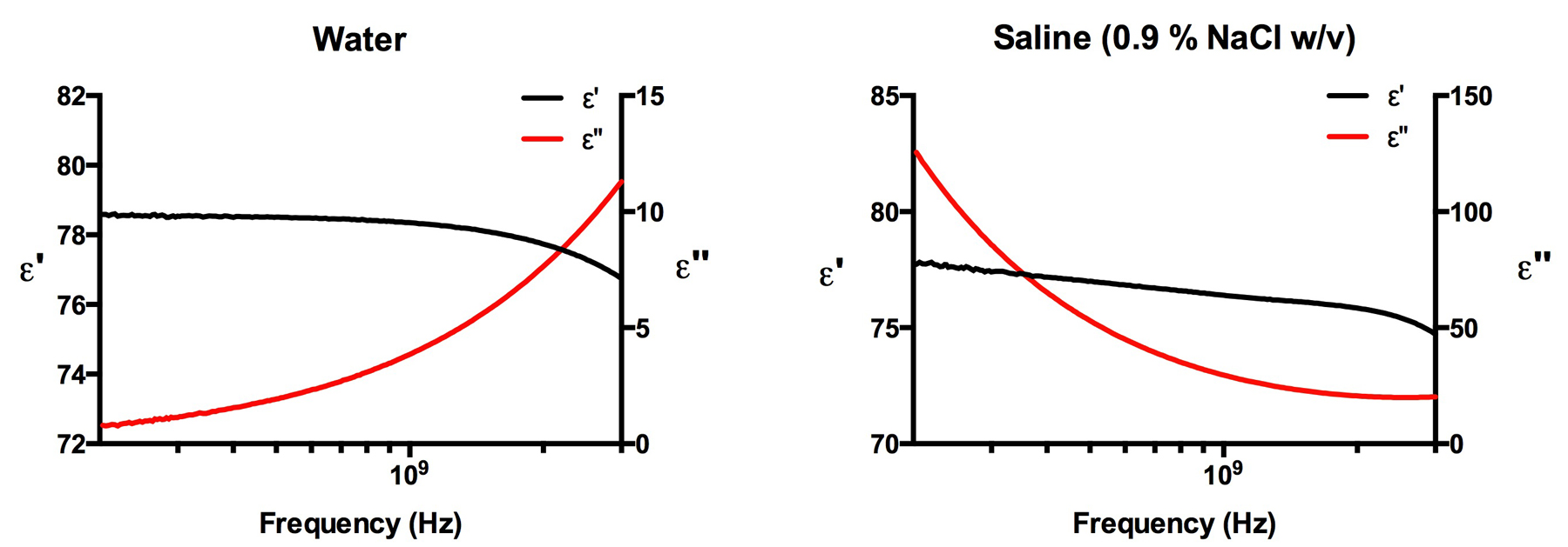
The data files extracted from the impedance analyzer and dielectric probe setup previously described can be opened using any standard data processing software such as Microsoft Excel. The data will appear in three columns, which will be labeled frequency (Hz), ε', and ε" (representing the real and imaginary components of the permittivity, respectively). Any graphing software can be used to create simple graphs of the complex permittivity versus frequency. In the example below (Figure \(\PageIndex{6}\) ) we have used Prism to graph the real and complex permittivity’s versus frequency (200 MHz – 3 GHz) for the water and saline samples. For this frequency range no error correction is needed. For the analysis of frequencies below 200 MHz down to 10 MHz, which can be achieved using the impedance analyzer and dielectric probe configuration, error correction algorithms are needed to take into account electrode polarization effects that skew and distort the data. Gach et al. cover these necessary algorithms that can be used if needed.