1.5: Kinetic Analysis Based on Differential Scanning Calorimetry Data

The procedure of kinetic analysis of a reaction based on DSC experiment data can be exemplified by the curing of an epoxy resin. The curing reaction involves the opening of the epoxy ring by amine and is accompanied by an exotherm, which is recorded on a differential scanning calorimeter. The fraction of the cured resin is directly proportional to the evolved heat quantity. The knowledge of how the conversion (that is, the fraction of the reacted resin) depends on time and temperature provided by DSC enables one, in studying actual epoxy binders, to optimize the conditions of their treatment and the forming of products, for example, a polymer composite material. It is worth noting that curing occurs without weight change. TG measurements are therefore inapplicable in this case.

Figure 5.1: Chemical structures of the epoxy diane resin based on bisphenol A.

It is well known [11], that, depending on the composition of reagents and process conditions, curing would occur as a one-stage as well as a two-stage process. In the present section both variants are considered.

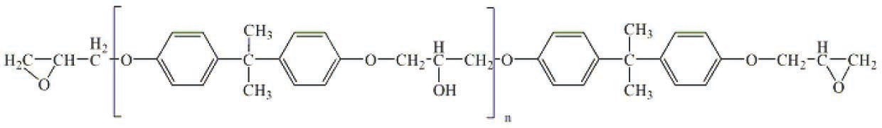
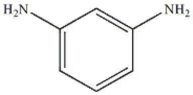
Let us consider a classical system consisting of an epoxy diane resin based on 4,4’-dihydroxydiphenylpropane (bisphenol A) (Figure 5.1) and a curing agent, metaphenylenediamine (Figure 5.2). The curing of this system was studied on a Netzsch DSC-204 Phenix analyzer. Measurements were taken at five heating rates: 2.5, 5, 7.5, 10, and 15 K/min. Samples were placed in Netzsch aluminum crucibles with a lid. A hole was preliminarily made in the lid. The process was carried out in an argon flow at a flow rate of 100 mL/min. A mixture of the resin components were freshly prepared before taking measurements. The samples were 5–5.5 mg for each of the heating rates.

Figure 5.2: Chemical structure of the curing agent, metaphenylenediamine.

5.1 Computation Procedure. Solution of the Inverse and Direct Kinetic Problems. Quasi-One-Stage Process

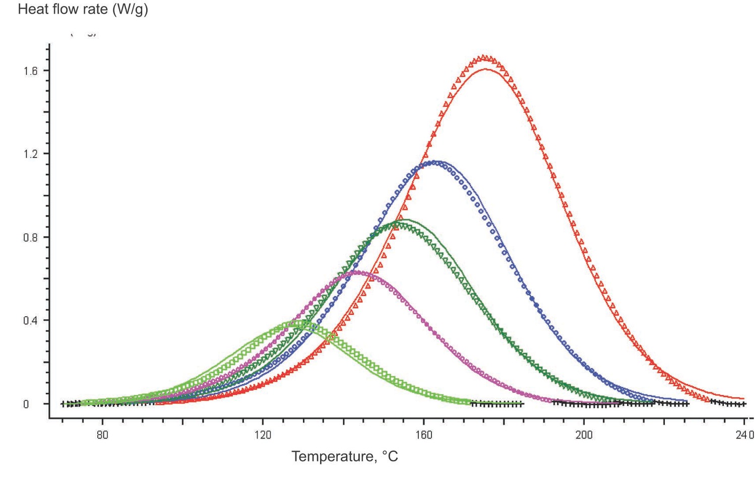
Experimental data acquired using the NETZSCH equipment is processed with the NETZSCH Proteus program. Figure 5.3 demonstrates that the curing of an epoxy resin in the given temperature range can be considered quasi-one-stage at all heating rates used.

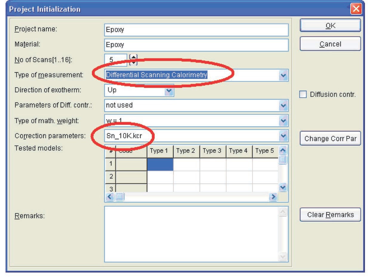
The procedure of kinetic analysis for DSC data is analogous to that for TG measurements described above. Here, we focus on the differences between these procedures. First of all, when loading data in the NETZSCH Thermokinetics software, the user select Differential Scanning Calorimetry as the type of measurement (Figure 5.4).

Figure 5.3: DSC curves of the curing of an epoxy resin at five heating rates.

Figure 5.4: Selection of the type of measurement for loading in the NETZSCH Thermokinetics software.

Figure 5.5: Example of the change in the peak shape for indium metal melting after the correction of the DSC signal (reprinted with permission from [9] © NETZSCH-Gerätebau GmbH).

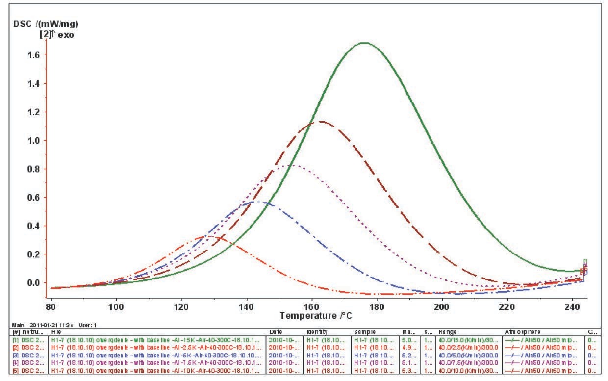
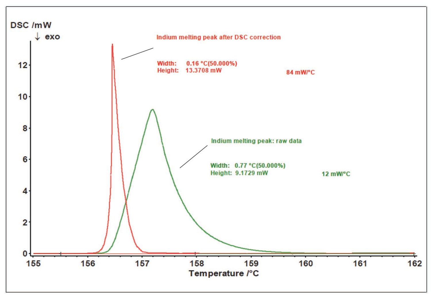
The DSC results not only provide information on the transformation of an analyte, but also depend on the heat exchange conditions in the analyzer–sample system. Because of the thermal resistance between the sample and the sensor, the thermal flow released as a result of processes in the sample is smeared in time (Figure 5.3). To correctly perform kinetic analysis, the true signal shape should be found, that is, data should be corrected for the time constant of the instrument and for thermal resistance. These corrections can be applied with the DSC Correction routine.

As a rule, the melting peak of pure metal (indium in this case) serves as the calibration measurement for determining the correction parameters. This metal is chosen because it melts in the same temperature range in which the epoxy resin is cured. The path to the file with preliminarily calculated correction parameters is specified in the same window (Figure 5.6).

Figure 5.6: Project initialization for DSC measurements.

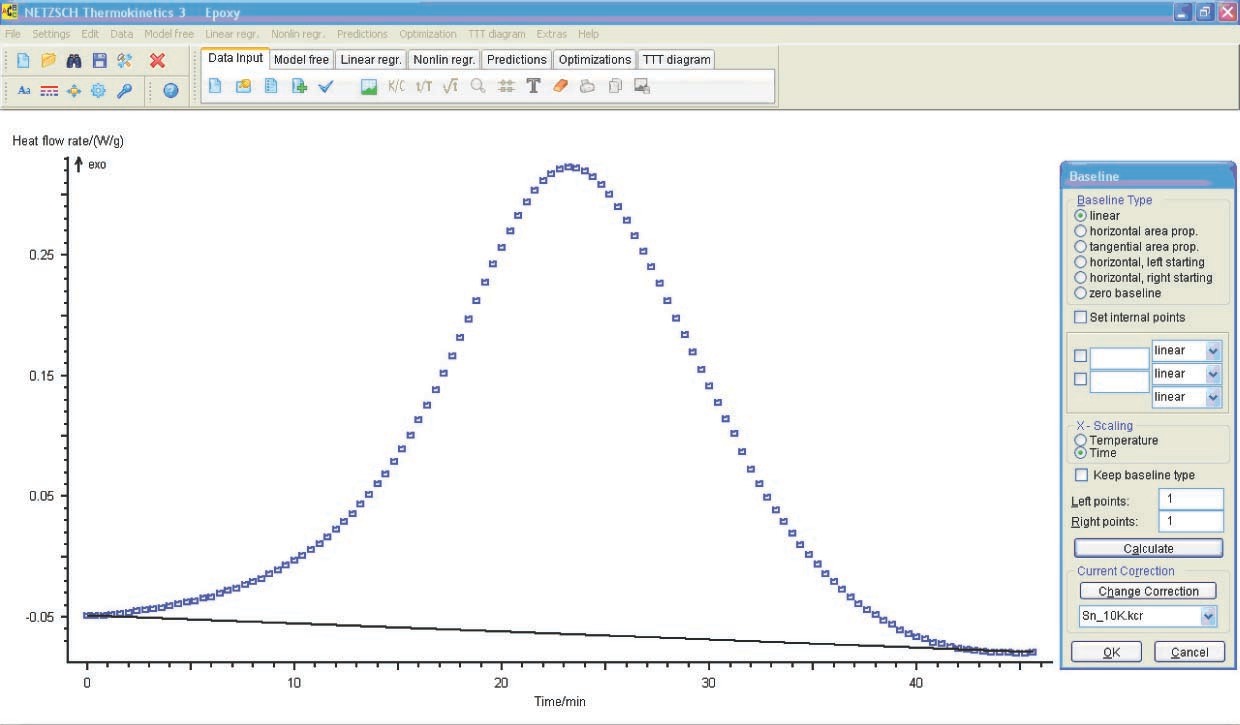
The data is loaded by clicking the Load ASCII file icon (see Figure 4.9), analogously to the procedure with TG data. If necessary, the user corrects the evaluation range limits (Figure 5.7). For further calculation, the type of baseline should be selected (Figure 5.8). In this case, we use a linear baseline.

Figure 5.7: Selection of the evaluation range limits in the NETZSCH Thermokinetics software.

Figure 5.8: Choice of the baseline.

The loaded data is checked and model-free analysis is performed (Figure 5.9).

Figure 5.9: Logarithm of heating rate versus inverse temperature (calculation by the Ozawa–Flynn–Wall method).

Figure 5.10: Activation energy and preexponential factor versus conversion (calculation by the Ozawa–Flynn–Wall method).

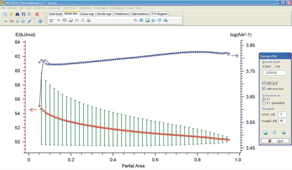
The resulting activation energies and preexponential factors are used as a zero approximation in solving the direct kinetic problem.

5.2 Analysis of Computation Results

Let us consider, first of all, the computation results (Figure 5.11) obtained by the linear regression method under the assumption of a one-stage process.

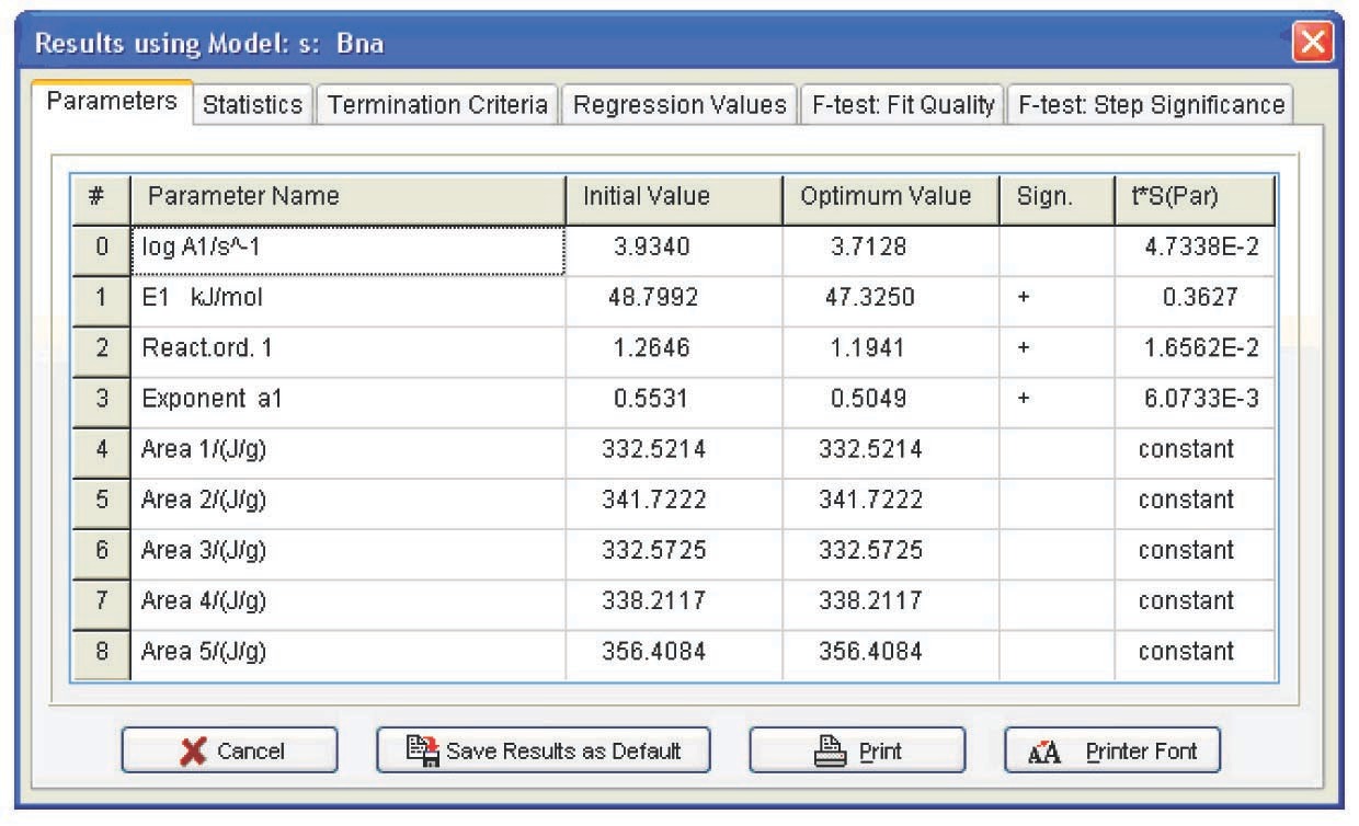
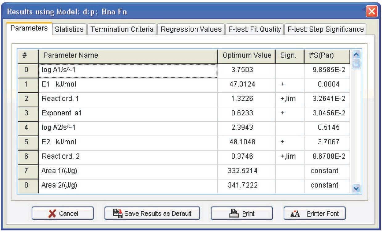
Figure 5.11 presents the Arrhenius parameters, the form of function, and its characteristics best fitting the experimental results (from the statistical viewpoint). The calculation was performed for all models. As expected, however, the only relevant model turned out to be the model of reaction with autocatalysis described by the Prout–Tompkins equation (Bna code) (Figure 5.12), which is indicated at the top left of the table showed in Figure 5.11.

Refinement of the model parameters by the nonlinear regression method led to results analogous to those in Figure 5.11. The statistical characteristics of the model are shown in Figure 5.13. With the inclusion of the Durbin–Watson test value, the resulting model parameters are as follows: E = 47 ± 3 kJ/mol, log A = 3.7 ± 0.4, n = 1.2 ± 0.15, a1 = 0.50 ± 0.05.

Figure 5.11: Arrhenius parameters obtained by non-linear regression.

Figure 5.12: Graphical comparison of the computation results (solid line) and experimental data (symbols) for DSC curves of the epoxy resin curing process. Five heating rates; one-step reaction; the Prout–Tompkins equation.

Figure 5.13: Statistical analysis of quality fits for different models.

As is known, the epoxy resin curing reaction occurs due to the autocatalysis mechanism [12]. The reaction is promoted by hydroxyl groups formed upon cross-linking [11]. At the early step of the reaction, the reaction rate increases with an increase in the conversion because of the catalytic effect of the reaction product. With a lapse of time, the amount of the starting reagent decreases, and so does the reaction rate. Thus, the plot of the reaction rate versus time passes through a maximum. In the simplest case, this mechanism is described by the Prout–Tompkins function, which also follows from our preliminary calculation. However, the curing process is known to comprise at least two independent steps. This function is therefore often unable to adequately describe the curing process. It is more preferable to use the following equation for calculation of the curing process [11]:

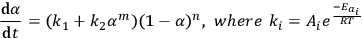
(5.1)

In the software, this equation is represented as a model with two parallel reactions: a reaction with autocatalysis described by the Prout–Tompkins equation (Bna) and an nth order equation (Fn).

Figure 5.14: Kinetic parameters for the two-step model.

Model with two parallel reactions: a reaction with autocatalysis described by the Prout–Tompkins equation and an nth order reaction (Fn). The kinetic parameters corresponding to a two-step model with two parallel reactions are presented in Figure 5.14. However, the difference between the fits provided by the one- and two-stage models is statistically insignificant, as follows from Figure 5.15. In both cases, the F_exp value does not exceed the critical value. We may assume that the one- and two-step processes are equiprobable. This phenomenon can be explained by the presence of hydroxyl groups in the initial resin: even at a zero conversion rate, catalytic sites exist, and the autocatalytic mechanism prevails during the entire course of the reaction.

Figure 5.15: Statistical analysis of the fit quality for different models.

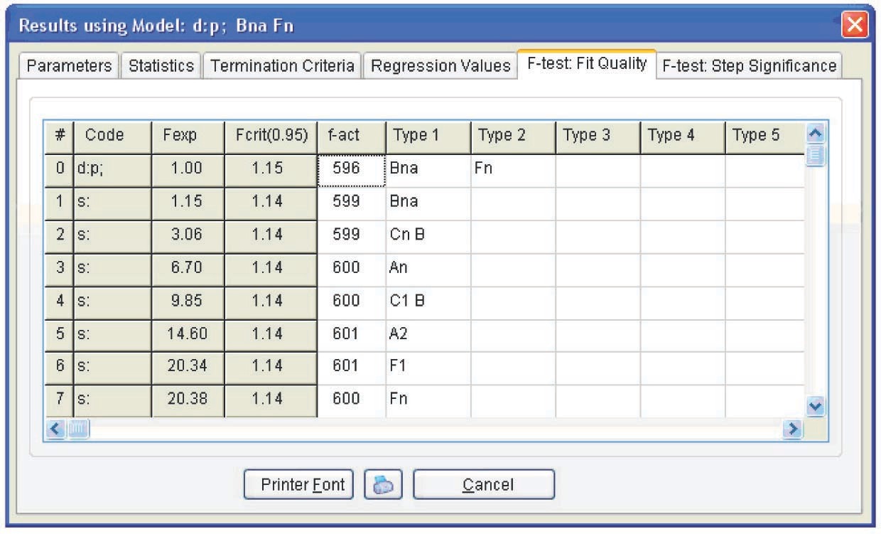
Table 5.1 presents the calculation results for both models. As is seen, the errors of the Fn function parameters for the two-stage process are significant, whereas the average parameter values do not differ from those of the Bna function. Hence, we can state that the above calculation does not confirm the occurrence of the two-stage curing process.

Function code	log A	E, kJ/mol	Reaction order n	Exp a1
Bna	7.7±0.4	47±3	1.2±0.15	0.50±0.05
Bna	3.75±0.7	47±6	1.3±0.2	0.6±0.2
Fn	2.4±5	48±26	0.4±0.6	—

5.1 Parameters for the one- and two-stage models.

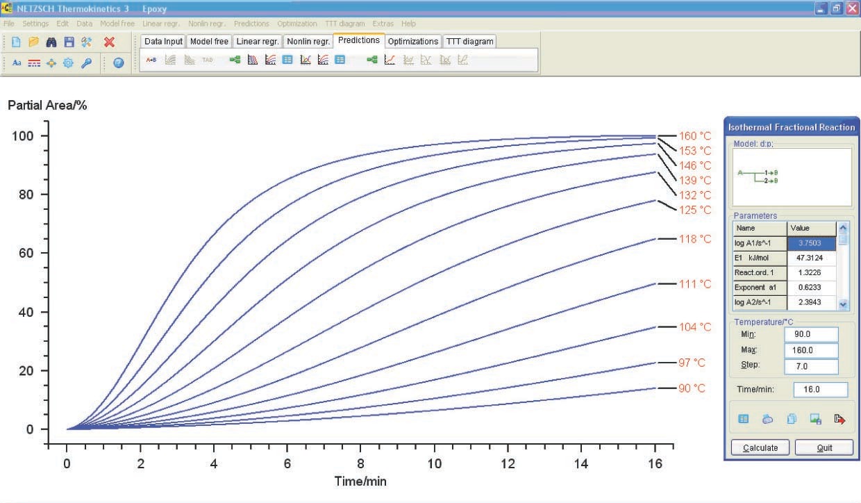
5.3 Plotting the Conversion-Time Curves

The above calculation can be successfully used for selecting optimal conditions for the curing process (temperature and time). Let us consider how to obtain the conversion versus time plot (at a given temperature) from the calculated data. To do this, we open the Predictions toolbar. The curves are shown in Figure 5.16. In this case, calculations are performed assuming the kinetic control of the reaction. In reality, once a certain curing degree has been achieved, the initially liquid sample is converted to the viscous flow and then to the solid state. The diffusion of resin and curing agent molecules thereby slows down, and the process becomes diffusion-controlled. Thus, the kinetic calculation should be completed with measurements of the rheological properties of the system. The resulting relationships show that the resin is completely cured within 16 min at 153 °C.

Figure 5.16: Degree of curing of the resin versus the time of exposure of the sample to constant temperature.