1.4: Kinetic Analysis Based on Thermogravimetry Data

4.1 Dehydration of Calcium Oxalate Monohydrate

Let us consider the dehydration as the reaction that occurs by the scheme , that is,

Figure 4.1 shows the TG curves of the dehydration of calcium oxalate monohydrate.

Figure 4.1: TG and DTG curves of the dehydration of calcium oxalate monohydrate at different heating rates.

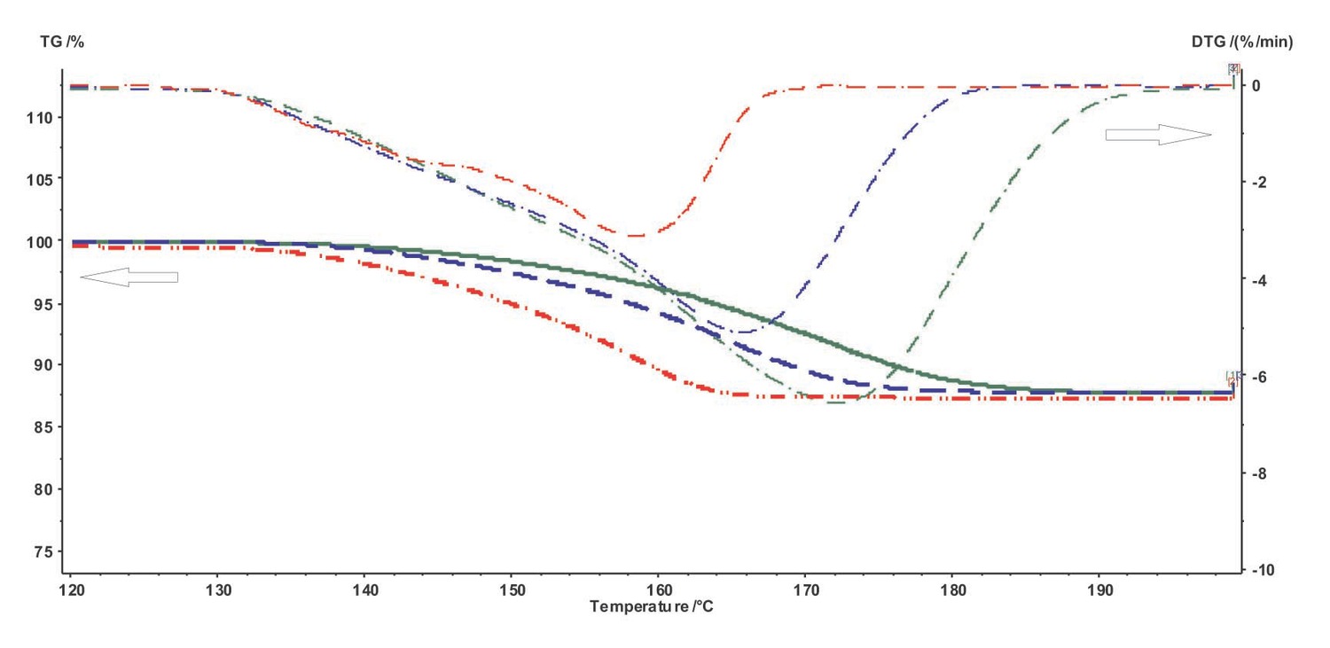
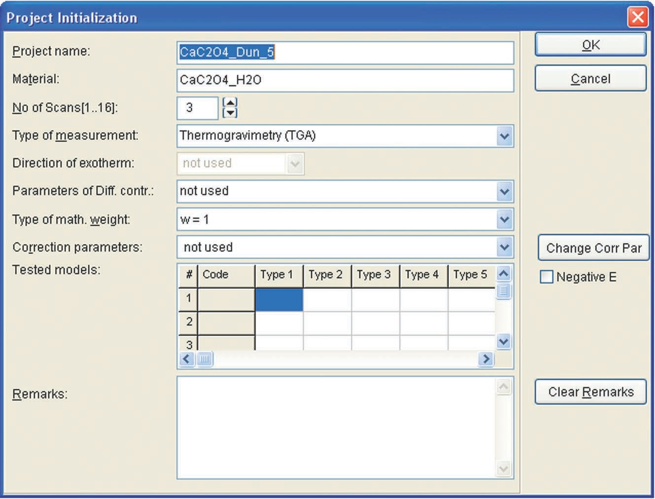
The CaC₂O₄ · H₂O dehydration was studied on a Netzsch TG 209 F 3 Tarsus thermo-microbalance. The experiment was run at three heating rates: 5, 7.5, and 10 K/min. Three measurements were taken at each heating rate, other conditions being identical. Standard aluminum crucibles without lids were used as holders. The process was carried out in a dry air flow at a rate of 200 mL/min. The initial reagent was freshly precipitated calcium oxalate with a particle size of 15–20 μm. Weighed portions of the reagent were 5–6 mg for each heating rate.

4.2 Computational Procedure. Solution of the Inverse and Direct Kinetic Problems. Quasi-One-Stage Process

As follows from Figure 4.1, the dehydration in the given temperature range can be considered a quasi-one-stage reaction at all heating rates used. The experimental data obtained on NETZSCH equipment are processed with the NETZSCH Proteus software.

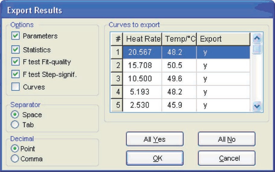
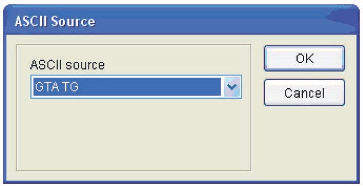
For further work with the experimental data using the NETZSCH Thermokinetics software, it is necessary to export data from the Proteus program in the tabulated form (measured signal as a function of temperature or time) as an ASCII file. To do this, the user must select the desired curve and click the Extras Export data button in the Proteus toolbar. The user must enter the lower and upper limits of the data range to be exported. To correctly specify the limits, the derivative of the selected curve is used. The left- and right-hand limits are chosen in the ranges where the derivative becomes zero (Figure 4.2).

Figure 4.2: Selection of the number of points while exporting data.

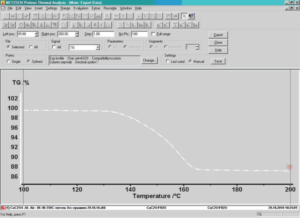
Remember that the derivative of the selected curve can be obtained by clicking the corresponding icon in the NETZSCH Proteus program window.

. For the selected temperature range, 100 points for each curve are used. It is worth noting that the use of a smaller increment is physically unreasonable since the S value reflects the properties of the system in question, but is not the temperature measurement accuracy provided by an instrument, which is an order of lower magnitude. In this case, specific features of the process should be taken into account.

Figure 4.4) is considered sufficient when the DTG curve has no spikes.

Figure 4.5). In the initialization dialog box, the project name, the sample, the number of measured curves (scans), and the type of measurement (TG, DSC, etc.) are entered.

Figure 4.8), the type of measurement is specified. In the case of thermogravimetry, GTA TG is selected.

Figure 4.9). In the popup window, the user specifies the desired data file.

Figure 4.10).

Figure 4.11).

Figure 4.12).

Figure 4.13).

Figure 4.15).

Figure 4.16). This procedure is applicable to one-step processes.

Figure 4.17). To do this, in the Selection box, the user should click on ‘Yes’ in the corresponding cell of the column ‘Selected’. The program outputs a graph of measured and calculated curves, as well as tables.

4.3 Analysis of Computation Results

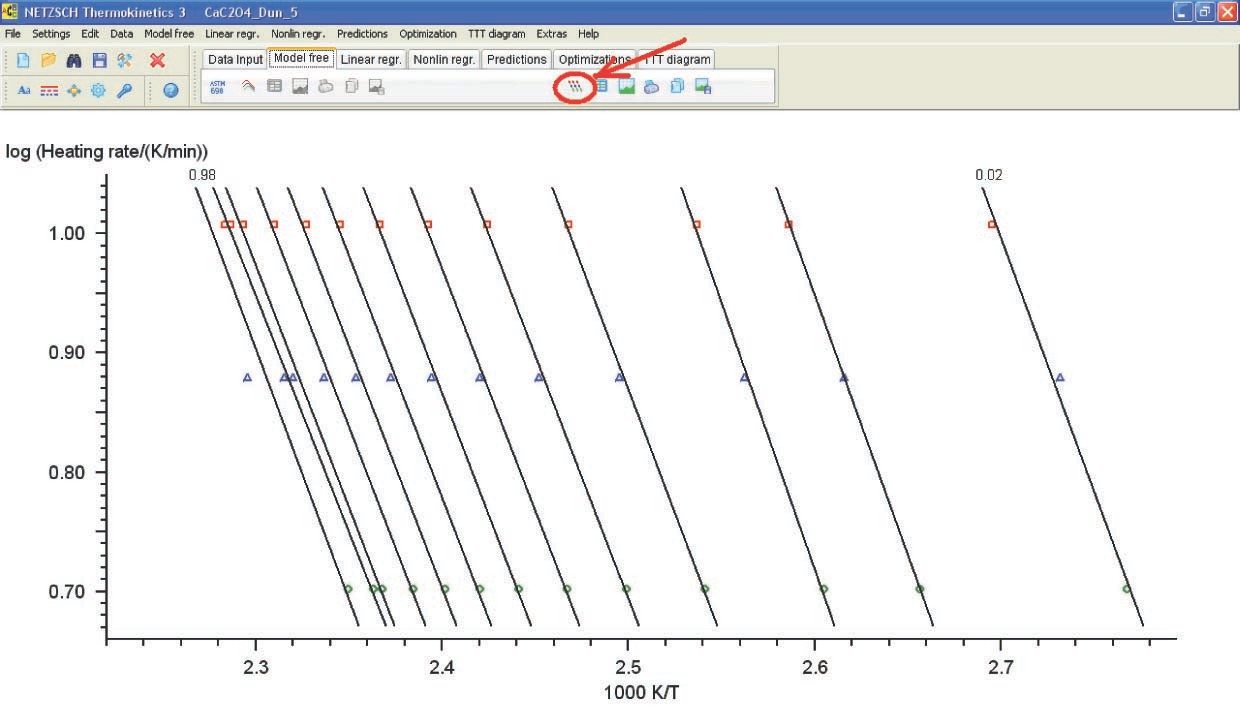
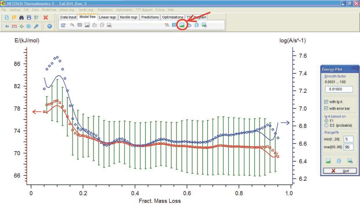
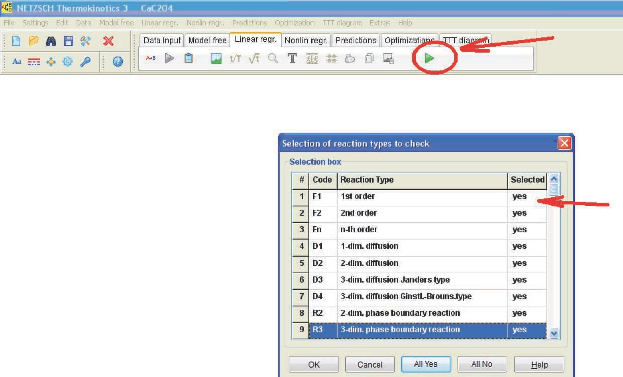
Let us consider the computation results obtained by the linear regression method for the CaC₂O₄ · H₂O dehydration (Figure 4.19).

Figure 4.19 presents the Arrhenius parameters and the form and characteristics of the function best fitting the experimental results (from the statistical viewpoint). For the reaction under consideration, the best fitting function is the Prout–Tompkins equation with autocatalysis (the Bna code), which is indicated at the top left of the table. However, before discussing the meaning of the results obtained, let us consider the F-test: Fit Quality window (Figure 4.20).

Figure 4.20: Fit quality for different models.

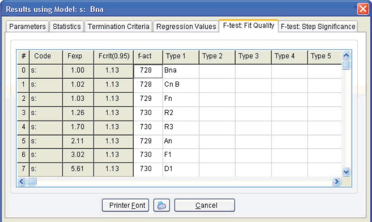
4.3.1 The F-test: Fit quality and F-test

Step significance windows present the statistical analysis of the fit quality for different models. This allows us to determine using the statistical methods which of the models provides the best fit for the experimental data.

To perform such an analysis, Fisher’s exact test is used. In general, Fisher’s test is a variance ratio which makes it possible to verify whether the difference between two independent estimates of the variance of some data samples is significant. To do this, the ratio of these two variances is compared with the corresponding tabulated value of the Fisher distribution for a given number of degrees of freedom and significance level. If the ratio of two variances exceeds the corresponding theoretical Fisher test value, the difference between the variances is significant.

In the Thermokinetics software, Fisher’s test is used for comparing the fit qualities ensured by different models. The best-fit model, that is, the model with the minimal sum of squared deviations, is taken as a reference (conventionally denoted as model 1). Then, each model is compared to the reference model. If the Fisher test value does not exceed the critical value, the difference between current model 2 and reference model 1 is insignificant. There is no reason to then believe that model 1 provides a more adequate description of the experiment in comparison to model 2.

The F_exp value is estimated by means of Fisher’s test:

\[F_{e x p}=\frac{L S Q_{1} / f_{1}}{L S Q_{2} / f_{2}} \label{4.2}\]

The F_exp value is compared with the Fisher distribution F_crit(0.95) for the significance level of 0.95 and the corresponding number of degrees of freedom.

Figure 4.21).

Figure 4.24).

In the Const. column, the option ‘false’ is set for the parameters that should be varied and the option ‘true’ is chosen for the parameters that remain constant. The three columns to the right of this column are intended for imposing constraints on the selected values. The computation results are presented in Figure 4.25.

Figure 4.25), the Durbin–Watson test value is presented (4.3) which should be added to the calculated tS error, where t is the Student’s test for a given number of degrees of freedom, and S is the mean-square deviation. Thus, we obtain the following set of parameters and their errors (Table 4.1) for all statistically equivalent functions.

Figure 4.26: Computation results for the Fn function.

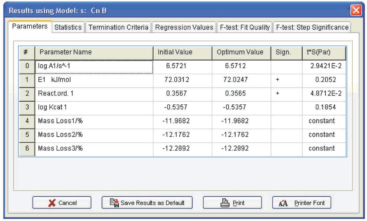
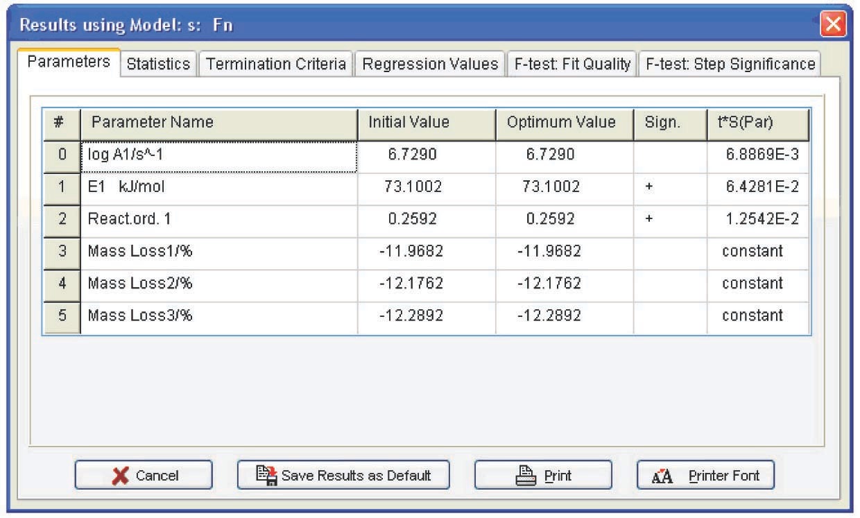
The following conclusions can be drawn from Table 4.1: first, the autocatalysis parameters for the Bna and CnB functions are almost zero, that is, all is reduced to the Fn function. Second, the error of the Arrhenius parameters for Fn are minimal. Hence, the calcium oxalate dehydration is better described by the nth-order function. The reaction order can be considered to be 1/3, that is, the process is described by the “contracting sphere equation.” This means that the sample consists of spherical particles of the same size and that the dehydration is a homothetic process, that is, the particles during decomposition undergo a self-similar decrease in size. Such a mechanism is inherent in thermolysis of inorganic crystal hydrates. Thus, the problem of CaC₂O₄·H₂O dehydration macrokinetics can be thought of as solved.

4.1 Kinetic parameters of the CaC2O4∙H2O dehydration process

Function code	log A	E, kJ/mol	Reaction order n	log K cat 1	Exp a1
Bna	6.8±0.6	73±6	0.34±0.25	—	0.06±0.14
CnB	6.8±1	74±8	0.41±0.48	-0.45±1.9	—
Fn	7.0±0.1	75.2±0.8	0.34±0.25	—	—

The project created in the NETZSCH Thermokinetics software is saved by clicking on the common button (Figure 4.27).

Figure 4.29).

Figure 4.29: Selection of data for export as an ASCII file.