11.7: Using R for a Multivariate Linear Regression

To illustrate how we can use R to complete a multivariate linear regression, use this link and save the file allSpec.csv to your working directory. The data in this file consists of 80 rows and 642 columns. Each row is an independent sample that contains one or more of the following transition metal cations: Cu²⁺, Co²⁺, Cr³⁺, and Ni²⁺. The first seven columns provide information about the samples:

• a sample id (in the form custd_1 for a single standard of Cu²⁺ or nicu_mix1 for a mixture of Ni²⁺ and Cu²⁺)
• a list of the analytes in the sample (in the form cuco for a sample that contains Cu²⁺ and Co²⁺)
• the number of analytes in the sample (a number from 1 to 4 and labeled as dimensions)
• the molar concentration of Cu²⁺ in the sample
• the molar concentration of Co²⁺ in the sample
• the molar concentration of Cr³⁺ in the sample
• the molar concentration of Ni²⁺ in the sample

The remaining columns contain absorbance values at 635 wavelengths between 380.5 nm and 899.5 nm. We will use a subset of this data that is identical to that used to illustrate a cluster analysis and a principal component analysis.

First, we need to read the data into R, which we do using the read.csv() function

spec_data <- read.csv("allSpec.csv", check.names = FALSE)

where the option check.names = FALSE overrides the function's default to not allow a column's name to begin with a number. Next, we will create objects to hold the concentrations and absorbances for standard solutions of Cu²⁺, Cr³⁺, and Co²⁺, which are the three analytes

wavelength_ids = seq(8, 642, 40)
abs_stds = spec_data[1:15, wavelength_ids]
conc_stds = data.frame(spec_data[1:15, 4], spec_data[1:15, 5], spec_data[1:15, 6])
abs_samples = spec_data[c(1, 6, 11, 21:25, 38:53), wavelength_ids]

where wavelength_ids is a vector that identifies the 16 equally spaced wavelengths, abs_stds is a data frame that gives the absorbance values for 15 standard solutions of the three analytes Cu²⁺, Cr³⁺, and Co²⁺ at the 16 wavelengths, conc_stds is a data frame that contains the concentrations of the three analytes in the 15 standard solutions, and abs_samples is a data frame that contains the absorbances of the 24 sample at the 16 wavelengths. This is the same data used to illustrate cluster analysis and principal component analysis.

To solve for the \(\epsilon b\) matrix we will write and source the following function that takes two objects—a data frame of absorbance values and a data frame of concentrations—and returns a matrix of \(\epsilon b\) values.

findeb = function(abs, conc){
abs.m = as.matrix(abs)
conc.m = as.matrix(conc)
ct = t(conc.m)
ctc = ct %*% conc.m
invctc = solve(ctc)
eb = invctc %*% ct %*% abs.m
output = eb
invisible(output)
}

Passing abs_stds and conc_stds to the function

eb_pred = findeb(abs_stds, conc_stds)

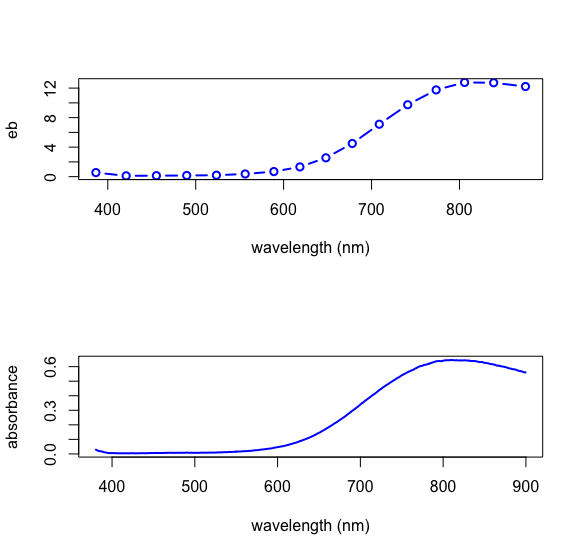
returns the predicted values for \(\epsilon b\) that make up our calibration. As we see below, a plot of the \(\epsilon b\) values for Cu²⁺ has the same shape as a plot of the absorbance values for one of the Cu²⁺ standards.

wavelengths = as.numeric(colnames(spec_data[8:642]))
old.par = par(mfrow = c(2,1))
plot(x = wavelengths[wavelength_ids], y = eb_pred[1,], type = "b",
xlab = "wavelength (nm)", ylab = "eb", lwd = 2, col = "blue")
plot(x = wavelengths, y = spec_data[1,8:642], type = "l",
xlab = "wavelength (nm)", ylab = "absorbance", lwd = 2, col = "blue")
par(old.par)

Having completed the calibration, we can determine the concentrations of the three analytes in the 24 samples using the following function, which takes as inputs thea data frame of absobance values and the \(\epsilon b\) matrix returned by the function findeb

findconc = function(abs, eb){
abs.m = as.matrix(abs)
eb.m = as.matrix(eb)
ebt = t(eb.m)
ebebt = eb %*% ebt
invebebt = solve(ebebt)
pred_conc = round(abs.m %*% ebt %*% invebebt, digits = 5)
output = pred_conc
invisible(output)
}
pred_conc = findconc(abs_samples, eb_pred)

To determine the error in the predicted concentrations, we first extract the actual concentrations from the original data set as a data frame, adjusting the column names for clarity.

real_conc = data.frame(spec_data[c(1, 6, 11, 21:25, 38:53), 4],
spec_data[c(1, 6, 11, 21:25, 38:53), 5],
spec_data[c(1, 6, 11, 21:25, 38:53), 6])
colnames(real_conc) = c("copper", "cobalt", "chromium")

and determine the difference between the actual concentrations and the predicted concentrations

conc_error = real_conc - pred_conc

Finally, we can report the mean error, the standard deviation, and the 95% confidence interval for each analyte.

means = apply(conc_error, 2, mean)
round(means, digits = 6)

copper cobalt chromium

-0.000280 -0.000153 -0.000210

sds = apply(conc_error, 2, sd)
round(sds, digits = 6)

copper cobalt chromium

0.001037 0.000811 0.000688

conf.it = abs(qt(0.05/2, 20)) * sds
round(conf.it, digits = 6)

copper cobalt chromium

0.002163 0.001693 0.001434

Compared to the ranges of concentrations for the three analytes in the 24 samples

range(real_conc$copper)

[1] 0.00 0.05

range(real_conc$cobalt)

[1] 0.0 0.1

range(real_conc$chromium)

[1] 0.0000 0.0375

the mean errors and confidence intervals are sufficiently small that we have confidence in the results.