
7.3: Analysis of Variance
- Page ID
- 222409

Consider the following data, which shows the stability of a reagent under different conditions for storing samples; all values are percent recoveries, so a result of 100 indicates that the reagent's concentration remains unchanged and that there was no degradation.
| trial/treatment | A (total dark) | B (subdued light) | C (full light) |
| 1 | 101 | 100 | 90 |
| 2 | 101 | 99 | 92 |
| 3 | 104 | 101 | 94 |
To determine if light has a significant affect on the reagent’s stability, we might choose to perform a series of t–tests, comparing all possible mean values; in this case we need three such tests:
- compare A to B
- compare A to C
- compare B to C
Each such test has a probability of a type I error of \(\alpha_{test}\). The total probability of a type I error across k tests, \(\alpha_{total}\), is
\[\alpha_{total} = 1 - (1 - \alpha_{test})^{k} \nonumber\]
For three such tests using \(\alpha = 0.05\), we have
\[\alpha_{total} = 1 - (1 - 0.05)^{3} = 0.143 \nonumber\]
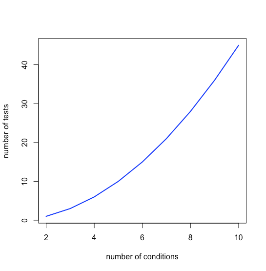
or a 14.3% proability of a type I error. The relationship between the number of conditions, n, and the number of tests, k, is
\[k = \frac {n(n-1)} {2} \nonumber\]
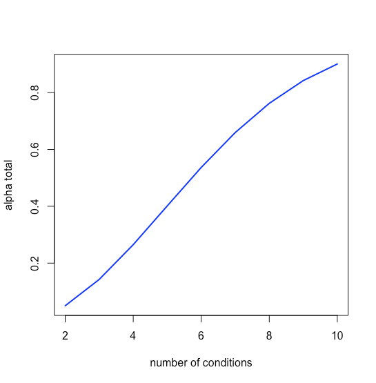
which means that k grows quickly as n increases, as shown in Figure \(\PageIndex{1}\).
and that the magnitude of a type I error increases quickly as well, as seen in Figure \(\PageIndex{2}\).
We can compensate for this problem by decreasing \(\alpha_{test}\) for each independent test so that \(\alpha_{total}\) is equal to our desired probability; thus, for \(n = 3\) we have \(k = 3\), and to achieve an \(\alpha_{total}\) of 0.05 each individual value of \(\alpha_{test}\) be
\[\alpha_{test} = 1 - (1 - 0.05)^{1/3} = 0.017 \nonumber\]
Values of \(\alpha_{test}\) decrease quickly, as seen in Figure \(\PageIndex{3}\).

The problem here is that we are searching for a significant difference on a pair-wise basis without any evidence that the overall variation in the data across all conditions (also known as treatments) is sufficiently large that it cannot be explained by experimental uncertainty (that is, random error) only. One way to determine if there is a systematic error in the data set, without identifying the source of the systematic error, is to compare the variation within each treatment to the variation between the treatments. We assume that the variation within each treatment reflects uncertainty in the analytical method (random errors) and that the variation between the treatments includes both the method’s uncertainty and any systematic errors in the individual treatments. If the variation between the treatments is significantly greater than the variation within the treatments, then a systematic error seems likely. We call this process an analysis of variance, or ANOVA; for one independent variable (the amount of light in this case), it is a one-way analysis of variance.
The basic details of a one-way ANOVA calculation are as follows:
Step 1: Treat the data as one large data set and calculate its mean and its variance, which we call the global mean, \(\bar{\bar{x}}\), and the global variance, \(\bar{\bar{s^{2}}}\).
\[\bar{\bar{x}} = \frac { \sum_{i=1}^h \sum_{j=1}^{n_{i}} x_{ij} } {N} \nonumber\]
\[\bar{\bar{s^{2}}} = \frac { \sum_{i=1}^h \sum_{j=1}^{n_{i}} (x_{ij} - \bar{\bar{x}})^{2} } {N - 1} \nonumber\]
where \(h\) is the number of treatments, \(n_{i}\) is the number of replicates for the \(i^{th}\) treatment, and \(N\) is the total number of measurements.
Step 2: Calculate the within-sample variance, \(s_{w}^{2}\), using the mean for each treatment, \(\bar{x}_{i}\), and the replicates for that treatment.
\[s_{w}^{2} = \frac { \sum_{i=1}^h \sum_{j=1}^{n_{i}} (x_{ij} - \bar{x}_{i})^{2} } {N - h} \nonumber\]
Step 3: Calculate the between-sample variance, \(s_{b}^{2}\), using the means for each treatment and the global mean
\[s_{b}^{2} = \frac { \sum_{i=1}^h \sum_{j=1}^{n_{i}} (\bar{x}_{i} - \bar{\bar{x}})^2 } {h - 1} = \frac {\sum_{i=1}^h n_{i} (\bar{x}_{i} - \bar{\bar{x}})^2 } {h - 1} \nonumber\]
Step 4: If there is a significant difference between the treatments, then \(s_{b}^{2}\) should be significantly greater than \(s_{w}^{2}\), which we evaluate using a one-tailed \(F\)-test where
\[H_{0}: s_{b}^{2} = s_{w}^{2} \nonumber\]
\[H_{A}: s_{b}^{2} > s_{w}^{2} \nonumber\]
Step 5: If there is a significant difference, then we estimate \(\sigma_{rand}^{2}\) and \(\sigma_{systematic}^{2}\) as
\[s_{w}^{2} \approx \sigma_{rand}^{2} \nonumber\]
\[s_{b}^{2} \approx \sigma_{rand}^{2} + \bar{n}\sigma_{systematic}^{2} \nonumber\]
where \(\bar{n}\) is the average number of replicates per treatment.
This seems like a lot of work, but we can simplify the calculations by noting that
\[SS_{total} = \sum_{i=1}^h \sum_{j=1}^{n_{i}} (x_{ij} - \bar{\bar{x}})^{2} = \bar{\bar{s^{2}}}(N - 1) \nonumber\]
\[SS_{w} = \sum_{i=1}^h \sum_{j=1}^{n_{i}} (x_{ij} - \bar{x}_{i})^{2} \nonumber\]
\[SS_{b} = \sum_{i=1}^h n_{i} (\bar{x}_{i} - \bar{\bar{x}})^2 \nonumber\]
\[SS_{total} = SS_{w} + SS_{b} \nonumber\]
and that \(SS_{total}\) and \(SS_{b}\) are relatively easy to calculate, where \(SS\) is short for sum-of-squares. Table \(\PageIndex{1}\) gathers these equations together
| source of variance | sum-of-squares | degrees of freedom | variance |
| between samples | \(\sum_{i=1}^h n_{i} (\bar{x}_{i} - \bar{\bar{x}})^2\) | \(h - 1\) | \(s_{b}^{2} = \frac {SS_{b}} {h - 1}\) |
| within samples | \(SS_{total} = SS_{w} + SS_{b}\) | \(N - h\) | \(s_{w}^{2} = \frac {SS_{w}} {N - h}\) |
| total | \(\bar{\bar{s^{2}}}(N - 1)\) |
Chemical reagents have a limited shelf-life. To determine the effect of light on a reagent's stability, a freshly prepared solution is stored for one hour under three different light conditions: total dark, subdued light, and full light. At the end of one hour, each solution was analyzed three times, yielding the following percent recoveries; a recovery of 100% means that the measured concentration is the same as the actual concentration.The null hypothesis is that there is there is no difference between the different treatments, and the alternative hypothesis is that at least one of the treatments yields a result that is significantly different than the other treatments.
| trial/condition | A (total dark) | B (subdued light) | C (full light) |
| 1 | 101 | 100 | 90 |
| 2 | 101 | 99 | 92 |
| 3 | 104 | 101 | 94 |
Solution
First, we treat the data as one large data set of nine values and calculate the global mean, \(\bar{\bar{x}}\), and the global variance, \(\bar{\bar{s^{2}}}\); these are 98 and 23.75, respectively. We also calculate the mean for each of the three treatments, obtaining a value of 102.0 for treatment A, 100.0 for treatment B, and 92.0 for treatment C.
Next, we calculate the total sum-of-squares, \(SS_{total}\)
\[\bar{\bar{s^{2}}}(N - 1) = 23.75(9 - 1) = 190.0 \nonumber\]
the between sample sum-of-squares, \(SS_{b}\)
\[SS_{b} = \sum_{i=1}^h n_{i} (\bar{x}_{i} - \bar{\bar{x}})^2 = 3(102.0 - 98.0)^2 + 3(100.0 - 98.0)^2 + 3(92.0 - 98.0)^2 = 168.0 \nonumber\]
and the within sample sum-of-squares, \(SS_{w}\)
\[ SS_{w} = SS_{total} - SS_{b} = 190.0 - 168.0 = 22.0 \nonumber\]
The variance between the treatments, \(s_b^2\) is
\[\frac {SS_{b}} {h - 1} = \frac{168}{3 - 1} = 84.0 \nonumber\]
and the variance within the treatments, \(s_w^2\) is
\[\frac {SS_{w}} {N - h} = \frac{22.0}{9 - 3} = 3.67 \nonumber\]
Finally, we complete an F-test, calculating Fexp
\[F_{exp} = \frac{s_b^2}{s_w^2} = \frac{84.0}{3.67} = 22.9 \nonumber\]
and compare it to the critical value for F(0.05, 2, 6) = 5.143 from Appendix 3. Because Fexp > F(0.05, 2, 6), we reject the null hypothesis and accept the alternative hypothesis that at least one of the treatments yields a result that is significantly different from the other treatments. We can estimate the variance due to random errors as
\[\sigma_{random}^{2} = s_{w}^{2} = 3.67 \nonumber\]
and the variance due to systematic errors as
\[\sigma_{systematic}^{2} = \frac {\sigma_{random}^{2} - s_{w}^{2}} {\bar{n}} = \frac {84.0 - 3.67} {3} = 26.8 \nonumber\]
Having found evidence for a significant difference between the treatments, we can use individual t-tests on pairs of treatments to show that the results for treatment C are significantly different from the other two treatments.