
7.1: Significance Testing
- Page ID
- 221818

Let’s consider the following problem. To determine if a medication is effective in lowering blood glucose concentrations, we collect two sets of blood samples from a patient. We collect one set of samples immediately before we administer the medication, and we collect the second set of samples several hours later. After we analyze the samples, we report their respective means and variances. How do we decide if the medication was successful in lowering the patient’s concentration of blood glucose?
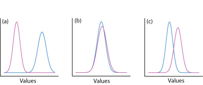
One way to answer this question is to construct a normal distribution curve for each sample, and to compare the two curves to each other. Three possible outcomes are shown in Figure \(\PageIndex{1}\). In Figure \(\PageIndex{1a}\), there is a complete separation of the two normal distribution curves, which suggests the two samples are significantly different from each other. In Figure \(\PageIndex{1b}\), the normal distribution curves for the two samples almost completely overlap each other, which suggests the difference between the samples is insignificant. Figure \(\PageIndex{1c}\), however, presents us with a dilemma. Although the means for the two samples seem different, the overlap of their normal distribution curves suggests that a significant number of possible outcomes could belong to either distribution. In this case the best we can do is to make a statement about the probability that the samples are significantly different from each other.
The process by which we determine the probability that there is a significant difference between two samples is called significance testing or hypothesis testing. Before we discuss specific examples let's first establish a general approach to conducting and interpreting a significance test.
Constructing a Significance Test
The purpose of a significance test is to determine whether the difference between two or more results is sufficiently large that we are comfortable stating that the difference cannot be explained by indeterminate errors. The first step in constructing a significance test is to state the problem as a yes or no question, such as
“Is this medication effective at lowering a patient’s blood glucose levels?”
A null hypothesis and an alternative hypothesis define the two possible answers to our yes or no question. The null hypothesis, H0, is that indeterminate errors are sufficient to explain any differences between our results. The alternative hypothesis, HA, is that the differences in our results are too great to be explained by random error and that they must be determinate in nature. We test the null hypothesis, which we either retain or reject. If we reject the null hypothesis, then we must accept the alternative hypothesis and conclude that the difference is significant.
Failing to reject a null hypothesis is not the same as accepting it. We retain a null hypothesis because we have insufficient evidence to prove it incorrect. It is impossible to prove that a null hypothesis is true. This is an important point and one that is easy to forget. To appreciate this point let’s use this data for the mass of 100 circulating United States pennies.
| Penny | Weight (g) | Penny | Weight (g) | Penny | Weight (g) | Penny | Weight (g) |
|---|---|---|---|---|---|---|---|
| 1 | 3.126 | 26 | 3.073 | 51 | 3.101 | 76 | 3.086 |
| 2 | 3.140 | 27 | 3.084 | 52 | 3.049 | 77 | 3.123 |
| 3 | 3.092 | 28 | 3.148 | 53 | 3.082 | 78 | 3.115 |
| 4 | 3.095 | 29 | 3.047 | 54 | 3.142 | 79 | 3.055 |
| 5 | 3.080 | 30 | 3.121 | 55 | 3.082 | 80 | 3.057 |
| 6 | 3.065 | 31 | 3.116 | 56 | 3.066 | 81 | 3.097 |
| 7 | 3.117 | 32 | 3.005 | 57 | 3.128 | 82 | 3.066 |
| 8 | 3.034 | 33 | 3.115 | 58 | 3.112 | 83 | 3.113 |
| 9 | 3.126 | 34 | 3.103 | 59 | 3.085 | 84 | 3.102 |
| 10 | 3.057 | 35 | 3.086 | 60 | 3.086 | 85 | 3.033 |
| 11 | 3.053 | 36 | 3.103 | 61 | 3.084 | 86 | 3.112 |
| 12 | 3.099 | 37 | 3.049 | 62 | 3.104 | 87 | 3.103 |
| 13 | 3.065 | 38 | 2.998 | 63 | 3.107 | 88 | 3.198 |
| 14 | 3.059 | 39 | 3.063 | 64 | 3.093 | 89 | 3.103 |
| 15 | 3.068 | 40 | 3.055 | 65 | 3.126 | 90 | 3.126 |
| 16 | 3.060 | 41 | 3.181 | 66 | 3.138 | 91 | 3.111 |
| 17 | 3.078 | 42 | 3.108 | 67 | 3.131 | 92 | 3.126 |
| 18 | 3.125 | 43 | 3.114 | 68 | 3.120 | 93 | 3.052 |
| 19 | 3.090 | 44 | 3.121 | 69 | 3.100 | 94 | 3.113 |
| 20 | 3.100 | 45 | 3.105 | 70 | 3.099 | 95 | 3.085 |
| 21 | 3.055 | 46 | 3.078 | 71 | 3.097 | 96 | 3.117 |
| 22 | 3.105 | 47 | 3.147 | 72 | 3.091 | 97 | 3.142 |
| 23 | 3.063 | 48 | 3.104 | 73 | 3.077 | 98 | 3.031 |
| 24 | 3.083 | 49 | 3.146 | 74 | 3.178 | 99 | 3.083 |
| 25 | 3.065 | 50 | 3.095 | 75 | 3.054 | 100 | 3.104 |
After looking at the data we might propose the following null and alternative hypotheses.
H0: The mass of a circulating U.S. penny is between 2.900 g and 3.200 g
HA: The mass of a circulating U.S. penny may be less than 2.900 g or more than 3.200 g
To test the null hypothesis we find a penny and determine its mass. If the penny’s mass is 2.512 g then we can reject the null hypothesis and accept the alternative hypothesis. Suppose that the penny’s mass is 3.162 g. Although this result increases our confidence in the null hypothesis, it does not prove that the null hypothesis is correct because the next penny we sample might weigh less than 2.900 g or more than 3.200 g.
After we state the null and the alternative hypotheses, the second step is to choose a confidence level for the analysis. The confidence level defines the probability that we will incorrectly reject the null hypothesis when it is, in fact, true. We can express this as our confidence that we are correct in rejecting the null hypothesis (e.g. 95%), or as the probability that we are incorrect in rejecting the null hypothesis. For the latter, the confidence level is given as \(\alpha\), where
\[\alpha = 1 - \frac {\text{confidence interval (%)}} {100} \nonumber\]
For a 95% confidence level, \(\alpha\) is 0.05.
The third step is to calculate an appropriate test statistic and to compare it to a critical value. The test statistic’s critical value defines a breakpoint between values that lead us to reject or to retain the null hypothesis, which is the fourth, and final, step of a significance test. As we will see in the sections that follow, how we calculate the test statistic depends on what we are comparing.
The four steps for a statistical analysis of data using a significance test:
- Pose a question, and state the null hypothesis, H0, and the alternative hypothesis, HA.
- Choose a confidence level for the statistical analysis.
- Calculate an appropriate test statistic and compare it to a critical value.
- Either retain the null hypothesis, or reject it and accept the alternative hypothesis.
One-Tailed and Two-tailed Significance Tests
Suppose we want to evaluate the accuracy of a new analytical method. We might use the method to analyze a Standard Reference Material that contains a known concentration of analyte, \(\mu\). We analyze the standard several times, obtaining a mean value, \(\overline{X}\), for the analyte’s concentration. Our null hypothesis is that there is no difference between \(\overline{X}\) and \(\mu\)
\[H_0 \text{: } \overline{X} = \mu \nonumber\]
If we conduct the significance test at \(\alpha = 0.05\), then we retain the null hypothesis if a 95% confidence interval around \(\overline{X}\) contains \(\mu\). If the alternative hypothesis is
\[H_\text{A} \text{: } \overline{X} \neq \mu \nonumber\]
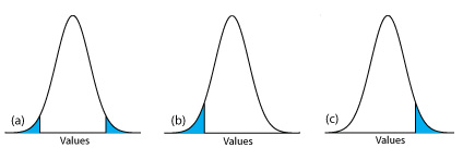
then we reject the null hypothesis and accept the alternative hypothesis if \(\mu\) lies in the shaded areas at either end of the sample’s probability distribution curve (Figure \(\PageIndex{2a}\)). Each of the shaded areas accounts for 2.5% of the area under the probability distribution curve, for a total of 5%. This is a two-tailed significance test because we reject the null hypothesis for values of \(\mu\) at either extreme of the sample’s probability distribution curve.
We can write the alternative hypothesis in two additional ways
\[H_\text{A} \text{: } \overline{X} > \mu \nonumber\]
\[H_\text{A} \text{: } \overline{X} < \mu \nonumber\]
rejecting the null hypothesis if \(\mu\) falls within the shaded areas shown in Figure \(\PageIndex{2b}\) or Figure \(\PageIndex{2c}\), respectively. In each case the shaded area represents 5% of the area under the probability distribution curve. These are examples of a one-tailed significance test.
For a fixed confidence level, a two-tailed significance test is the more conservative test because rejecting the null hypothesis requires a larger difference between the results we are comparing. In most situations we have no particular reason to expect that one result must be larger (or must be smaller) than the other result. This is the case, for example, when we evaluate the accuracy of a new analytical method. A two-tailed significance test, therefore, usually is the appropriate choice.
We reserve a one-tailed significance test for a situation where we specifically are interested in whether one result is larger (or smaller) than the other result. For example, a one-tailed significance test is appropriate if we are evaluating a medication’s ability to lower blood glucose levels. In this case we are interested only in whether the glucose levels after we administer the medication are less than the glucose levels before we initiated treatment. If a patient’s blood glucose level is greater after we administer the medication, then we know the answer—the medication did not work—and we do not need to conduct a statistical analysis.
Errors in Significance Testing
Because a significance test relies on probability, its interpretation is subject to error. In a significance test, \(\alpha\) defines the probability of rejecting a null hypothesis that is true. When we conduct a significance test at \(\alpha = 0.05\), there is a 5% probability that we will incorrectly reject the null hypothesis. This is known as a type 1 error, and its risk is always equivalent to \(\alpha\). A type 1 error in a two-tailed or a one-tailed significance tests corresponds to the shaded areas under the probability distribution curves in Figure \(\PageIndex{2}\).
A second type of error occurs when we retain a null hypothesis even though it is false. This is a type 2 error, and the probability of its occurrence is \(\beta\). Unfortunately, in most cases we cannot calculate or estimate the value for \(\beta\). The probability of a type 2 error, however, is inversely proportional to the probability of a type 1 error.
Minimizing a type 1 error by decreasing \(\alpha\) increases the likelihood of a type 2 error. When we choose a value for \(\alpha\) we must compromise between these two types of error. Most of the examples in this text use a 95% confidence level (\(\alpha = 0.05\)) because this usually is a reasonable compromise between type 1 and type 2 errors for analytical work. It is not unusual, however, to use a more stringent (e.g. \(\alpha = 0.01\)) or a more lenient (e.g. \(\alpha = 0.10\)) confidence level when the situation calls for it.