6.1: Properties of a Normal Distribution

Last updated
Save as PDF

Page ID: 220899

\( \newcommand{\vecs}[1]{\overset { \scriptstyle \rightharpoonup} {\mathbf{#1}} } \) \( \newcommand{\vecd}[1]{\overset{-\!-\!\rightharpoonup}{\vphantom{a}\smash {#1}}} \)\(\newcommand{\id}{\mathrm{id}}\) \( \newcommand{\Span}{\mathrm{span}}\) \( \newcommand{\kernel}{\mathrm{null}\,}\) \( \newcommand{\range}{\mathrm{range}\,}\) \( \newcommand{\RealPart}{\mathrm{Re}}\) \( \newcommand{\ImaginaryPart}{\mathrm{Im}}\) \( \newcommand{\Argument}{\mathrm{Arg}}\) \( \newcommand{\norm}[1]{\| #1 \|}\) \( \newcommand{\inner}[2]{\langle #1, #2 \rangle}\) \( \newcommand{\Span}{\mathrm{span}}\) \(\newcommand{\id}{\mathrm{id}}\) \( \newcommand{\Span}{\mathrm{span}}\) \( \newcommand{\kernel}{\mathrm{null}\,}\) \( \newcommand{\range}{\mathrm{range}\,}\) \( \newcommand{\RealPart}{\mathrm{Re}}\) \( \newcommand{\ImaginaryPart}{\mathrm{Im}}\) \( \newcommand{\Argument}{\mathrm{Arg}}\) \( \newcommand{\norm}[1]{\| #1 \|}\) \( \newcommand{\inner}[2]{\langle #1, #2 \rangle}\) \( \newcommand{\Span}{\mathrm{span}}\)\(\newcommand{\AA}{\unicode[.8,0]{x212B}}\)

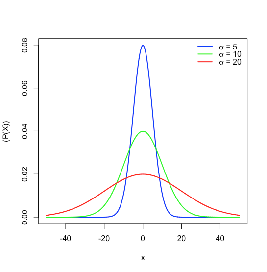
Mathematically a normal distribution is defined by the equation

\[P(x) = \frac {1} {\sqrt{2 \pi \sigma^2}} e^{-(x - \mu)^2/(2 \sigma^2)} \nonumber\]

where \(P(x)\) is the probability of obtaining a result, \(x\), from a population with a known mean, \(\mu\), and a known standard deviation, \(\sigma\). Figure \(\PageIndex{1}\) shows the normal distribution curves for \(\mu = 0\) with standard deviations of 5, 10, and 20.

Figure \(\PageIndex{1}\): Three examples of normal distribution curves. Although the height and width are affected by \(\sigma\), the area under each curve is the same.

Because the equation for a normal distribution depends solely on the population’s mean, \(\mu\), and its standard deviation, \(\sigma\), the probability that a sample drawn from a population has a value between any two arbitrary limits is the same for all populations. For example, Figure \(\PageIndex{2}\) shows that 68.26% of all samples drawn from a normally distributed population have values within the range \(\mu \pm 1\sigma\), and only 0.14% have values greater than \(\mu + 3\sigma\).

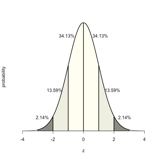
Figure \(\PageIndex{2}\): Normal distribution curve for \(\mu = 0\) and \(\sigma = 1\) showing area under the curve for various values of \(z\) in \(\mu \pm z \sigma\).

This feature of a normal distribution—that the area under the curve is the same for all values of \(\sigma\)—allows us to create a probability table (see Appendix 1) based on the relative deviation, \(z\), between a limit, x, and the mean, \(\mu\).

\[z = \frac {x - \mu} {\sigma} \nonumber\]

The value of \(z\) gives the area under the curve between that limit and the distribution’s closest tail, as shown in Figure \(\PageIndex{3}\).

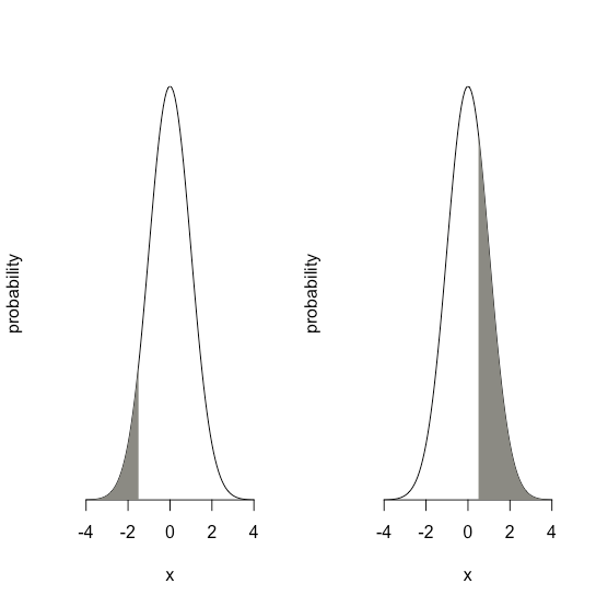
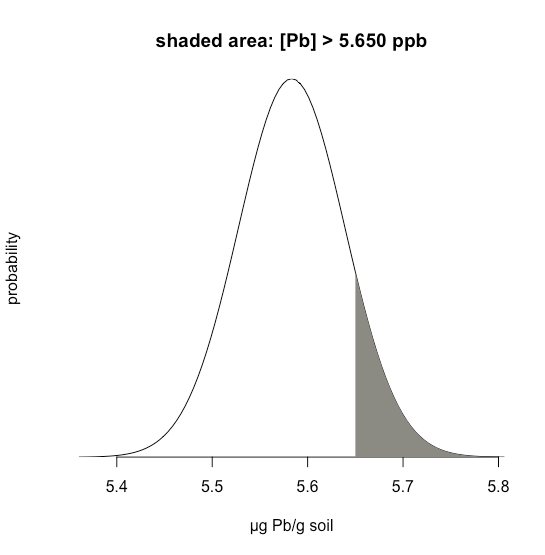
Figure \(\PageIndex{3}\): Normal distribution curve for \(\mu = 0\) and \(\sigma = 1\) showing (on the left) the area under the curve for \(z = −1.5\) and (on the right for \(z = +0.5\).

Example \(\PageIndex{1}\)

Suppose we know that \(\mu\) is 5.5833 ppb Pb and that \(\sigma\) is 0.0558 ppb Pb for a particular standard reference material (SRM). What is the probability that we will obtain a result that is greater than 5.650 ppb if we analyze a single, random sample drawn from the SRM?

Solution

Figure \(\PageIndex{4}\) shows the normal distribution curve given values of 5.5833 ppb Pb for \(\mu\) and of 0.0558 ppb Pb \(\sigma\). The shaded area in the figures is the probability of obtaining a sample with a concentration of Pb greater than 5.650 ppm. To determine the probability, we first calculate \(z\)

\[z = \frac {x - \mu} {\sigma} = \frac {5.650 - 5.5833} {0.0558} = 1.195 \nonumber\]

Next, we look up the probability in Appendix 1 for this value of \(z\), which is the average of 0.1170 (for \(z = 1.19\)) and 0.1151 (for \(z = 1.20\)), or a probability of 0.1160; thus, we expect that 11.60% of samples will provide a result greater than 5.650 ppb Pb.

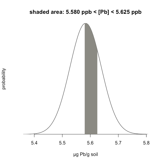
Figure \(\PageIndex{4}\): Normal distribution curve for the amount of lead in a standard reference with \(\mu = 5.5833\) ppb and \(\sigma = 0.0558\) ppb. The shaded area shows those results for which the concentration of lead exceeds 5.650 ppb.

Example \(\PageIndex{2}\)

Example \(\PageIndex{1}\) considers a single limit—the probability that a result exceeds a single value. But what if we want to determine the probability that a sample has between 5.580 g Pb and 5.625 g Pb?

Solution

In this case we are interested in the shaded area shown in Figure \(\PageIndex{5}\). First, we calculate \(z\) for the upper limit

\[z = \frac {5.625 - 5.5833} {0.0558} = 0.747 \nonumber\]

and then we calculate \(z\) for the lower limit

\[z = \frac {5.580 - 5.5833} {0.0558} = -0.059 \nonumber\]

Then, we look up the probability in Appendix 1 that a result will exceed our upper limit of 5.625, which is 0.2275, or 22.75%, and the probability that a result will be less than our lower limit of 5.580, which is 0.4765, or 47.65%. The total unshaded area is 71.4% of the total area, so the shaded area corresponds to a probability of

\[100.00 - 22.75 - 47.65 = 100.00 - 71.40 = 29.6 \% \nonumber\]

Figure \(\PageIndex{5}\): Normal distribution curve for the amount of lead in a standard reference with \(\mu = 5.5833\) ppb and \(\sigma = 0.0558\) ppb. The shaded area shows those results for which the concentration of lead is more than 5.580 ppb and less than 5.625 ppb.