5.3: The Central Limit Theorem

Last updated
Save as PDF

Page ID: 219089

\( \newcommand{\vecs}[1]{\overset { \scriptstyle \rightharpoonup} {\mathbf{#1}} } \) \( \newcommand{\vecd}[1]{\overset{-\!-\!\rightharpoonup}{\vphantom{a}\smash {#1}}} \)\(\newcommand{\id}{\mathrm{id}}\) \( \newcommand{\Span}{\mathrm{span}}\) \( \newcommand{\kernel}{\mathrm{null}\,}\) \( \newcommand{\range}{\mathrm{range}\,}\) \( \newcommand{\RealPart}{\mathrm{Re}}\) \( \newcommand{\ImaginaryPart}{\mathrm{Im}}\) \( \newcommand{\Argument}{\mathrm{Arg}}\) \( \newcommand{\norm}[1]{\| #1 \|}\) \( \newcommand{\inner}[2]{\langle #1, #2 \rangle}\) \( \newcommand{\Span}{\mathrm{span}}\) \(\newcommand{\id}{\mathrm{id}}\) \( \newcommand{\Span}{\mathrm{span}}\) \( \newcommand{\kernel}{\mathrm{null}\,}\) \( \newcommand{\range}{\mathrm{range}\,}\) \( \newcommand{\RealPart}{\mathrm{Re}}\) \( \newcommand{\ImaginaryPart}{\mathrm{Im}}\) \( \newcommand{\Argument}{\mathrm{Arg}}\) \( \newcommand{\norm}[1]{\| #1 \|}\) \( \newcommand{\inner}[2]{\langle #1, #2 \rangle}\) \( \newcommand{\Span}{\mathrm{span}}\)\(\newcommand{\AA}{\unicode[.8,0]{x212B}}\)

Suppose we have a population for which one of its properties has a uniform distribution where every result between 0 and 1 is equally probable. If we analyze 10,000 samples we should not be surprised to find that the distribution of these 10000 results looks uniform, as shown by the histogram on the left side of Figure \(\PageIndex{1}\). If we collect 1000 pooled samples—each of which consists of 10 individual samples for a total of 10,000 individual samples—and report the average results for these 1000 pooled samples, we see something interesting as their distribution, as shown by the histogram on the right, looks remarkably like a normal distribution. When we draw single samples from a uniform distribution, each possible outcome is equally likely, which is why we see the distribution on the left. When we draw a pooled sample that consists of 10 individual samples, however, the average values are more likely to be near the middle of the distribution’s range, as we see on the right, because the pooled sample likely includes values drawn from both the lower half and the upper half of the uniform distribution.

Figure \(\PageIndex{1}\): Distribution of results when analyzing samples of size n = 1 (left) and samples of size n = 10 (right) drawn from a uniform distribution.

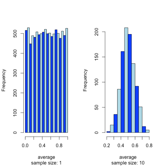
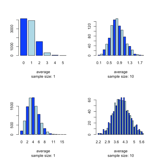
This tendency for a normal distribution to emerge when we pool samples is known as the central limit theorem. As shown in Figure \(\PageIndex{2}\), we see a similar effect with populations that follow a binomial distribution or a Poisson distribution.

Figure \(\PageIndex{2}\): Distribution of results when analyzing samples of size \(n = 1\) (left) and samples of size \(n = 10\) (right) drawn from a binomial distribution with p = 0.167 (top) and a Poisson distribution with \(\lambda = 4\) (bottom).

You might reasonably ask whether the central limit theorem is important as it is unlikely that we will complete 1000 analyses, each of which is the average of 10 individual trials. This is deceiving. When we acquire a sample of soil, for example, it consists of many individual particles each of which is an individual sample of the soil. Our analysis of this sample, therefore, is the mean for a large number of individual soil particles. Because of this, the central limit theorem is relevant.