5.2: Theoretical Models for the Distribution of Data
- Page ID
- 219088

There are four important types of distributions that we will consider in this chapter: the uniform distribution, the binomial distribution, the Poisson distribution, and the normal, or Gaussian, distribution. In Chapter 3 and Chapter 4 we used the analysis of bags of M&Ms to explore ways to visualize data and to summarize data. Here we will use the same data set to explore the distribution of data.
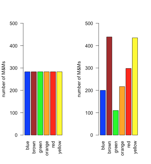
Uniform Distribution
In a uniform distribution, all outcomes are equally probable. Suppose the population of M&Ms has a uniform distribution. If this is the case, then, with six colors, we expect each color to appear with a probability of 1/6 or 16.7%. Figure \(\PageIndex{1}\) shows a comparison of the theoretical results if we draw 1699 M&Ms—the total number of M&Ms in our sample of 30 bags—from a population with a uniform distribution (on the left) to the actual distribution of the 1699 M&Ms in our sample (on the right). It seems unlikely that the population of M&Ms has a uniform distribution of colors!
Binomial Distribution
A binomial distribution shows the probability of obtaining a particular result in a fixed number of trials, where the odds of that result happening in a single trial are known. Mathematically, a binomial distribution is defined by the equation
\[P(X, N) = \frac {N!} {X! (N - X)!} \times p^{X} \times (1 - p)^{N - X} \nonumber\]
where P(X,N) is the probability that the event happens X times in N trials, and where p is the probability that the event happens in a single trial. The binomial distribution has a theoretical mean, \(\mu\), and a theoretical variance, \(\sigma^2\), of
\[\mu = Np \quad \quad \quad \sigma^2 = Np(1 - p) \nonumber\]
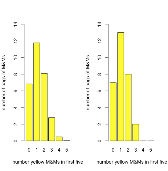
Figure \(\PageIndex{2}\) compares the expected binomial distribution for drawing 0, 1, 2, 3, 4, or 5 yellow M&Ms in the first five M&Ms—assuming that the probability of drawing a yellow M&M is 435/1699, the ratio of the number of yellow M&Ms and the total number of M&Ms—to the actual distribution of results. The similarity between the theoretical and the actual results seems evident; in Chapter 6 we will consider ways to test this claim.
Poisson Distribution
The binomial distribution is useful if we wish to model the probability of finding a fixed number of yellow M&Ms in a sample of M&Ms of fixed size—such as the first five M&Ms that we draw from a bag—but not the probability of finding a fixed number of yellow M&Ms in a single bag because there is some variability in the total number of M&Ms per bag.
A Poisson distribution gives the probability that a given number of events will occur in a fixed interval in time or space if the event has a known average rate and if each new event is independent of the preceding event. Mathematically a Poisson distribution is defined by the equation
\[P(X, \lambda) = \frac {e^{-\lambda} \lambda^X} {X !} \nonumber\]
where \(P(X, \lambda)\) is the probability that an event happens X times given the event’s average rate, \(\lambda\). The Poisson distribution has a theoretical mean, \(\mu\), and a theoretical variance, \(\sigma^2\), that are each equal to \(\lambda\).
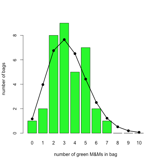
The bar plot in Figure \(\PageIndex{3}\) shows the actual distribution of green M&Ms in 35 small bags of M&Ms (as reported by M. A. Xu-Friedman “Illustrating concepts of quantal analysis with an intuitive classroom model,” Adv. Physiol. Educ. 2013, 37, 112–116). Superimposed on the bar plot is the theoretical Poisson distribution based on their reported average rate of 3.4 green M&Ms per bag. The similarity between the theoretical and the actual results seems evident; in Chapter 6 we will consider ways to test this claim.
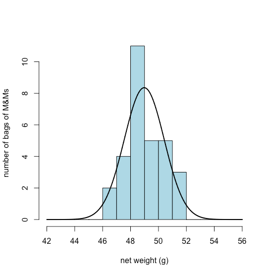
Normal Distribution
A uniform distribution, a binomial distribution, and a Poisson distribution predict the probability of a discrete event, such as the probability of finding exactly two green M&Ms in the next bag of M&Ms that we open. Not all of the data we collect is discrete. The net weights of bags of M&Ms is an example of continuous data as the mass of an individual bag is not restricted to a discrete set of allowed values. In many cases we can model continuous data using a normal (or Gaussian) distribution, which gives the probability of obtaining a particular outcome, P(x), from a population with a known mean, \(\mu\), and a known variance, \(\sigma^2\). Mathematically a normal distribution is defined by the equation
\[P(x) = \frac {1} {\sqrt{2 \pi \sigma^2}} e^{-(x - \mu)^2/(2 \sigma^2)} \nonumber\]
Figure \(\PageIndex{4}\) shows the expected normal distribution for the net weights of our sample of 30 bags of M&Ms if we assume that their mean, \(\overline{X}\), of 48.98 g and standard deviation, s, of 1.433 g are good predictors of the population’s mean, \(\mu\), and standard deviation, \(\sigma\). Given the small sample of 30 bags, the agreement between the model and the data seems reasonable.