3.3: Creating Plots From Scratch in R Using Base Graphics

Last updated
Save as PDF

Page ID: 219073

$ \newcommand{\vecs}[1]{\overset { \scriptstyle \rightharpoonup} {\mathbf{#1}} } $ $ \newcommand{\vecd}[1]{\overset{-\!-\!\rightharpoonup}{\vphantom{a}\smash {#1}}} $$\newcommand{\id}{\mathrm{id}}$ $ \newcommand{\Span}{\mathrm{span}}$ $ \newcommand{\kernel}{\mathrm{null}\,}$ $ \newcommand{\range}{\mathrm{range}\,}$ $ \newcommand{\RealPart}{\mathrm{Re}}$ $ \newcommand{\ImaginaryPart}{\mathrm{Im}}$ $ \newcommand{\Argument}{\mathrm{Arg}}$ $ \newcommand{\norm}[1]{\| #1 \|}$ $ \newcommand{\inner}[2]{\langle #1, #2 \rangle}$ $ \newcommand{\Span}{\mathrm{span}}$ $\newcommand{\id}{\mathrm{id}}$ $ \newcommand{\Span}{\mathrm{span}}$ $ \newcommand{\kernel}{\mathrm{null}\,}$ $ \newcommand{\range}{\mathrm{range}\,}$ $ \newcommand{\RealPart}{\mathrm{Re}}$ $ \newcommand{\ImaginaryPart}{\mathrm{Im}}$ $ \newcommand{\Argument}{\mathrm{Arg}}$ $ \newcommand{\norm}[1]{\| #1 \|}$ $ \newcommand{\inner}[2]{\langle #1, #2 \rangle}$ $ \newcommand{\Span}{\mathrm{span}}$$\newcommand{\AA}{\unicode[.8,0]{x212B}}$

As we saw in the last section, the functions to create dot charts, stripcharts, boxplots, barplots, and histograms have arguments that we can use to alter the appearance of the function’s output. For example, here is the full list of arguments available when we use dotchart()that control what the plot shows.

dotchart(x, labels = NULL, groups = NULL, gdata = NULL, cex = par("cex"), pt.cex = cex, pch = 21, gpch = 21, bg = par("bg"), color = par("fg"), gcolor = par("fg"), lcolor = "gray", xlim = range(x[is.finite(x)]), main = NULL, xlab = NULL, ylab = NULL, ...)

Each of the arguments has a default value, which means we need not specify the value for an argument unless we wish to change its value, as we did when we set pch to 19. The final argument of ... indicates that we can change any of a long list of graphical parameters that control what we see when we use dotchart.

Creating a Simple Scatterplot Using R

One of the most common, and most important, visualizations in analytical chemistry is a scatterplot in which we are interested in the relationship, if any, between two measurement by plotting the values for one variable along the x-axis and the values for the other variable along y-axis. For this exercise, we will use some data from the Puget Sound Data Hoard that gives the mass and the diameter for 816 M&Ms obtained from a 14.0-oz bag of plain M&Ms, a 12.7-oz bag of peanut M&Ms, and a 12.7-oz bag of peanut butter M&Ms. Let’s read the data into R and store it in a data frame with the name psmm_data. You can download a copy of the data using this link saving it in your working directory.

psmm_data = read.csv("data/PugetSoundM&MData.csv")

We might expect that as the diameter of an M&M increases so will the mass of the M&M. We might also expect that the relationship between diameter and mass may depend on whether the M&Ms are plain, peanut, or peanut butter. So that we can access data for each type of M&M, let’s use the which() function to create vectors that designate the row numbers for each of the three types of M&Ms.

pb_id = which(psmm_data$type == "peanut butter")

plain_id = which(psmm_data$type == "plain")

peanut_id = which(psmm_data$type == "peanut")

Typically we are interested in how one variable affects the other variable. We call the former the independent variable and place it on the x-axis and we call the latter the dependent variable and place it on the y-axis. Here we will use diameter as the independent variable and mass as the dependent variable. To create a scatterplot for the plain M&Ms we use the function plot(x, y) where x is the data to plot on the x-axis and y is the data to plot on the y-axis.

plot(x = psmm_data$diameter[plain_id], y = psmm_data$mass[plain_id])

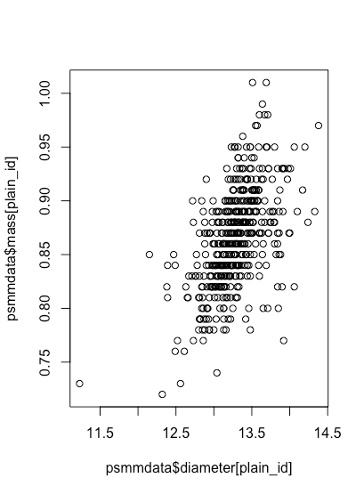
Figure $\PageIndex{1}$: A simple scatterplot created using R's `plot()` function.

Customizing a Plot Created Using R

Although our scatterplot shows that the mass of a plain M&M increases as its diameter increases, it is not a particularly attractive plot. In addition to specifying x and y, the plot function allows us to pass additional arguments to customize our plot; here are some of these optional arguments:

type = “option”. This argument specifies how points are displayed; there are a number of options, but the most useful are “p” for points (this is the default), “l” for lines without points, “b” for both points and lines that do not touch the points, “o” for points and lines that pass through the points, “h” for histogram-like vertical lines, and “s” for stair steps; use “n” if you wish to suppress the points.

pch = number. This argument selects the symbol used to plot the data, with the number assigned to each symbol shown below. The default option is 1, or an open circle. Symbols 15–20 are filled using the color of the symbol’s boundary, and symbols 21–25 can take a background color that is different from the symbol’s boundary. See later in this document for more details about setting colors. The figure below shows the different options.

# code from http://www.sthda.com/english/wiki/r-...available-in-r oldPar = par() par(font = 2, mar = c(0.5, 0, 0, 0)) y = rev(c(rep(1, 6),rep(2, 5), rep(3, 5), rep(4, 5), rep(5, 5))) x = c(rep(1:5, 5), 6) plot(x, y, pch = 0:25, cex = 1.5, ylim = c(1, 5.5), xlim = c(1, 6.5), axes = FALSE, xlab = "", ylab = "", bg = "blue") text(x, y, labels = 0:25, pos = 3) par(mar = oldPar$mar, font = oldPar$font)

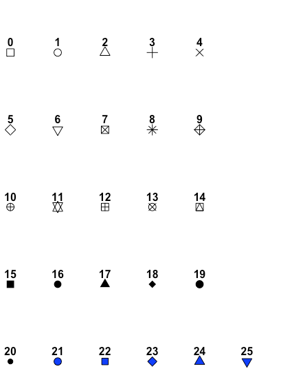
Figure $\PageIndex{2}$: The 25 `pch` symbols available in R's base graphics.

lty = number. This argument specifies the type of line to draw; the options are 1 for a solid line (this is the default), 2 for a dashed line, 3 for a dotted line, 4 for a dot-dash line, 5 for a long-dash line, and 6 for a two-dash line.

lwd = number. This argument sets the width of the line. The default is 1 and any other entry simply scales the width relative to the default; thus lwd = 2 doubles the width and lwd = 0.5 cuts the width in half.

bty = “option”. This argument specifies the type of box to draw around the plot; the options are “o” to draw all four sides (this is the default), “l” to draw on the left side and the bottom side only, “7” to draw on the top side and the right side only, “c” to draw all but the right side, “u” to draw all but the top side, “]” to draw all but the left side, and “n” to omit all four sides.

axes = logical. This argument indicates whether the axes are drawn (TRUE) or not drawn (FALSE); the default is TRUE.

xlim = c(begin, end). This argument sets the limits for the x-axis, overriding the default limits set by the plot() command.

ylim = c(begin, end). This argument sets the limits for the y-axis, overriding the default limits set by the plot() command.

xlab = “text”. This argument specifies the label for the x-axis, overriding the default label set by the plot() command.

ylab = “text”. This argument specifies the label for the y-axis, overriding the default label set by the plot() command.

main = “text”. This argument specifies the main title, which is placed above the plot, overriding the default title set by the plot() command.

sub = “text”. This argument specifies the subtitle, which is placed below the plot, overriding the default subtitle set by the plot() command.

cex = number. This argument controls the relative size of the symbols used to plot points. The default is 1 and any other entry simply scales the size relative to the default; thus cex = 2 doubles the size and cex = 0.5 cuts the size in half.

cex.axis = number. This argument controls the relative size of the text used for the scale on both axes; see the entry above for cex for more details.

cex.lab = number. This argument controls the relative size of the text used for the label on both axes; see the entry above for cex for more details.

cex.main = number. This argument controls the relative size of the text used for the plot’s main title; see the entry above for cex for more details.

cex.sub = number. This argument controls the relative size of the text used for the plot’s subtitle; see the entry above for cex for more details.

col = number or “string”. This argument controls the color of the symbols used to plot points. There are 657 available colors, for which the default is “black” or 24. You can see a list of colors (number and text string) by typing colors() in the console.

col.axis = number or “string”. This argument controls the color of the text used for the scale on both axes; see the entry above for col for more details.

col.lab = number or “string”. This argument controls the color of the text used for the label on both axes; see the entry above for col for more details.

col.main = number or “string”. This argument controls the color of the text used for the plot’s main title; see the entry above for col for more details.

col.sub = number or “string”. This argument controls the color of the text used for the plot’s subtitle; see the entry above for col for more details.

bg = number or “string”. This argument sets the background color for the plot symbols 21–25; see the entries above for pch and for col for more details.

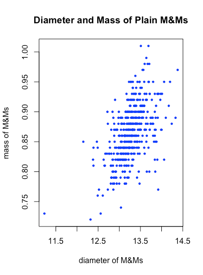
Let’s use some of these arguments to improve our scatterplot by adding some color to and adjusting the size of the symbols used to plot the data, and by adding a title and some more informative labels for the two axes.

plot(x = psmm_data$diameter[plain_id], y = psmm_data$mass[plain_id], xlab = "diameter of M&Ms", ylab = "mass of M&Ms", main = "Diameter and Mass of Plain M&Ms", pch = 19, cex = 0.5, col = "blue")

Figure $\PageIndex{3}$: An improved version of the scatterplot from Figure $\PageIndex{1}$.

Modifying an Existing Plot Created Using R

We can modify an existing plot in a number of useful ways, such as adding a new set of data, adding a reference line, adding a legend, adding text, and adding a set of grid lines; here are some of the things we can do:

points(x, y, . . . ). This command is identical to the plot() command, but overlays the new points on the current plot instead of first erasing the previous plot. Note: the points() command can not re-scale the axes; thus, you must ensure that your original plot—created using the plot() command—has x-axis and y-axis limits that meet your needs.

abline(h = number, . . . ). This command adds a horizontal line at y = number with the line’s color, type, and size set using the optional arguments.

abline(v = number, . . . ). This command adds a vertical line at x = number with the line’s color, type, and size set using the optional arguments.

abline(b = number, a = number, . . . ). This command adds a diagonal line defined by a slope (b) and a y-intercept (a); the line’s color, type, and size are set using the optional arguments. As we will see in Chapter 8, this is a useful command for displaying the results of a linear regression.

legend(location, legend, . . . ). This command adds a legend to the current plot. The location is specified in one of two ways:

• by giving the x and y coordinates for the legend’s upper-left corner using x = number and y = number)

• by using location = “keyword” where the keyword is one of “topleft”, “top”, “topright”, “right”, “bottomright”, “bottom”, “bottomleft”, or “left”; the optional argument inset = numbermoves the legend in from the margin when using a keyword (it takes a value from 0 to 1 as a fraction of the plot’s area; the default is 0)

The legend is added as a vector of character strings (one for each item in the legend), and any accompanying formatting, such as plot symbols, lines, or colors, are passed along as vectors of the same length; look carefully at the example at the end of this section to see how this command works.

text(location, label, . . . ). This command adds the text given by “label” to the current plot. The location is specified by providing values for x and y using x = number and y = number. By default, the text is centered at its location; to set the text so that it is left-justified (which is easier to work with), add the argument adj = c(0, NA).

grid(col, lty, lwd). This command adds a set of grid lines to the plot using the color, line type, and line width defined by “col”, “lty”, and “lwd”, respectively.

Here is an example of a figure in which we show how the diameter and mass vary as a function of the type of M&Ms, add a legend, add a grid, and add some text that identifies the source of the data. Note the use of the functions max and min to identify the limits needed to display results for all of the data.

# determine minimum and maximum values for diameter and mass so that we can

# set limits for the x-axis and y-axis that will allow plotting of all data

xmax = max(psmm_data$diameter)

xmin = min(psmm_data$diameter)

ymax = max(psmm_data$mass)

ymin = min(psmm_data$mass)

# create the initial plot using data for plain M&Ms, xlim and ylim values

# ensure plot window will allow plotting of all data

plot(x = psmm_data$diameter[plain_id], y = psmm_data$mass[plain_id], xlab = "diameter of M&Ms", ylab = "mass of M&Ms", main = "Diameter and Mass of M&Ms", pch = 19, cex = 0.65, col = "red", xlim = c(xmin, xmax), ylim = c(ymin, ymax))

# add the data for the peanut and peanut butter M&Ms using points()

points(x = psmm_data$diameter[peanut_id], y = psmm_data$mass[peanut_id], pch = 18, col = "brown", cex = 0.65)

points(x = psmm_data$diameter[pb_id], y = psmm_data$mass[pb_id], pch = 17, col = "blue", cex = 0.65)

# add a legend, gird, and explanatory text

legend(x = "topleft", legend = c("plain", "peanut", "peanut butter"), col = c("red", "brown", "blue"), pch = c(19, 18, 17), bty = "n")

grid(col = "gray")

text(x = 16.5, y = 1, label = "data from University of Puget Sound Data Hoard", cex = 0.5)

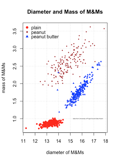
Figure $\PageIndex{4}$: Example of a more informative scatterplot.

Our new plot shows that the individual M&Ms are reasonably well separated from each other in the space created by the variables diameter and mass, although a few M&Ms encroach into the space occupied by other types of M&Ms. We also see that the distribution of plain M&Ms is much more compact than for peanut and peanut butter M&Ms, which makes sense given the likely variability in the size of individual peanuts and the softer consistency of peanut butter.