
1.2: The Basics of Working With R
- Page ID
- 218845

Communicating With R
The symbol > in the console is the command prompt, which indicates that R is awaiting your instructions. When you type a command in the console and hit Enter or Return, R executes the command and displays any appropriate output in the console; thus, this command adds the numbers 1 and 3
1 + 3
and returns the number 4 as an answer.
[1] 4
The text above is a code block that contains the line of code to enter into the console and the output generated by R. The command prompt (>) is not included here so that you can, if you wish, copy and paste the code into R; if you are copying and pasting the code, do not include the output or R will return an error message. Note that the output here is preceded by the number 1 in brackets, which is the id number of the first value returned on that line.
This is all well and good, but it is even less useful than a calculator because we cannot operate further on the result. If we assign this calculation to an object using an assignment operator, then the result of the calculation remains available to us.
There are two common leftward assignment operators in R: an arrow that points from right-to-left, <-, which means the value on the right is assigned to the object on the left, and an equals sign, =. Most style guides for R favor <- over =, but as = is the more common option in most other programming languages—such as Python, C++, and Matlab—we will use it here.
If we assign our calculation to the object answer then the result of the calculation is assigned to the object but not returned to us. To see an object’s value we can look for it in RStudio’s Environment Panel or enter the object’s name as a command in the Console, as shown here.
answer = 1 + 3
answer
[1] 4
Note that an object’s name is case-sensitive so answer and Answer are different objects.
Answer = 2 + 4
Answer
[1] 6
There are just a few limitations to the names you can assign to objects: they can include letters (both upper and lower case), numbers, dots (.), or underscores (_), but not spaces. A name can begin with a letter or with a dot followed by a letter (but not a dot followed by a number). Here are some examples of valid names
answerone answer_one answer1 answerOne answer.one
and examples of invalid names
1stanswer answer* first answer
You will find it helpful to use names that remind you of the object's meaning and that are not overly long. My personal preference is to use all lowercase letters, to use a descriptive noun, and to separate words using an underscore as I find that these choices make my code easier to read. When I find it useful to use the same base name for several objects of different types, then I may append a two or three letter designation to the name similar to the extensions that designate, for example, a spreadsheet stored as a .csv file. For example, when I use R to run a linear regression based on Beer's law, I may store the concentrations and absorbances of my standards in a data frame (see below for a description of data frames) with a name such as zinc.df and store the output of the linear model (see Chapter 8 for a discussion of linear models) in an object with a name such as zinc.lm.
Objects for Storing Data
In the code above, answer and Answer are objects that store a single numerical value. There are several different types of objects we can use to store data, including vectors, data frames, matrices and arrays, and lists.
Vectors
A vector is an ordered collection of elements of the same type, which may be numerical values, integer values, logical values, or character strings. Note that ordered does not imply that the values are arranged from smallest-to-largest or from largest-to-smallest, or in alphabetical order; it simply means the vector’s elements are stored in the order in which we enter them into the object. The length of a vector is the number of elements it holds. The objects answer and Answer, for example, are vectors with lengths of 1.
length(answer)
[1] 1
Most of the vectors we will use include multiple elements. One way to create a vector with multiple elements is to use the concatenation function, c( ).
In the code blocks below and elsewhere, any text that follows a hashtag, #, is a comment that explains what the line of code is accomplishing; comments are not executable code, so R simply ignores them.
For example, we can create a vector of numerical values,
v00 = c(1.1, 2.2, 3.3)
v00
[1] 1.1 2.2 3.3
or a vector of integers,
v01 = c(1, 2, 3)
v01
[1] 1 2 3
or a vector of logical values,
v02 = c(TRUE, TRUE, FALSE) # we also could enter this as c(T, T, F)
v02
[1] TRUE TRUE FALSE
or a vector of character strings
v03 = c("alpha", "bravo", "charley")
v03
[1] "alpha" "bravo" "charley"
You can view an object’s structure by examining it in the Environment Panel or by using R’s structure command, str( ) which, for example, identifies vector the v02 as a logical vector with an index for its entries of 1, 2, and 3, and with values of TRUE, TRUE, and FALSE.
str(v02)
logi [1:3] TRUE TRUE FALSE
We can use a vector’s index to correct errors, to add additional values, or to create a new vector using already existing vectors. Note that the number within the square brackets, [ ], identifies the element in the vector of interest. For example, the correct spelling for the third element in v03 is charlie, not charley; we can correct this using the following line of code.
v03[3] = "charlie" # correct the vector's third value
v03
[1] "alpha" "bravo" "charlie"
We can also use the square bracket to add a new element to an existing vector,
v00[4] = 4.4 # add a fourth element to the existing vector, increasing its length
v00
[1] 1.1 2.2 3.3 4.4
or to create a new vector using elements from other vectors.
v04 = c(v01[1], v02[2], v03[3])
v04
[1] "1" "TRUE" "charlie"
Note the the elements of v04 are character strings even though v01 contains integers and v02 contains logical values. This is because the elements of a vector must be of the same type, so R coerces them to a common type, in this case a vector of character strings.
Here are several ways to create a vector when its entries follow a defined sequence, seq( ), or use a repetitive pattern, rep( ).
v05 = seq(from = 0, to = 20, by = 4)
v05
[1] 0 4 8 12 16 20
v06 = seq(0, 10, 2) # R assumes the values are provided in the order from, to, and by
v06
[1] 0 2 4 6 8 10
v07 = rep(1:4, times = 2) # repeats the pattern 1, 2, 3, 4 twice
v07
[1] 1 2 3 4 1 2 3 4
v08 = rep(1:4, each = 2) # repeats each element in the string twice before proceeding to next element
v08
[1] 1 1 2 2 3 3 4 4
Note that 1:4 is equivalent to c(1, 2, 3, 4) or seq(1, 4, 1). In R it often is the case that there are multiple ways to accomplish the same thing!
Finally, we can complete mathematical operations using vectors, make logical inquiries of vectors, and create sub-samples of vectors.
v09 = v08 - v07 # subtract two vectors, which must be of equal length
v09
[1] 0 -1 -1 -2 2 1 1 0
v10 = (v09 == 0) # returns TRUE for each element in v10 that equals zero
v10
[1] TRUE FALSE FALSE FALSE FALSE FALSE FALSE TRUE
v11 = which(v09 < 1) # returns the index for each elements in v09 that is less than 1
v11
[1] 1 2 3 4 8
v12 = v09[!v09 < 1] # returns values for elements in v09 whose values are not less than 1
v12
[1] 2 1 1
Data Frames
A data frame is a collection of vectors—all equal in length but not necessarily of a single type of element—arranged with the vectors as the data frame's columns.
df01 = data.frame(v07, v08, v09, v10)
df01
v07 v08 v09 v10
1 1 1 0 TRUE
2 2 1 -1 FALSE
3 3 2 -1 FALSE
4 4 2 -2 FALSE
5 1 3 2 FALSE
6 2 3 1 FALSE
7 3 4 1 FALSE
8 4 4 0 TRUE
We can access the elements in a data frame using the data frame's index, which takes the form [row number(s), column number(s}], where [ is the bracket operator.
df02 = df01[1, ] # returns all elements in the data frame's first row
df02
v07 v08 v09 v10
1 1 1 0 TRUE
df03 = df01[ , 3:4] # returns all elements in the data frame's third and fourth columns
df03
v09 v10
1 0 TRUE
2 -1 FALSE
3 -1 FALSE
4 -2 FALSE
5 2 FALSE
6 1 FALSE
7 1 FALSE
8 0 TRUE
df04 = df01[4, 3] # returns the element in the data frame's fourth row and third column
df04
[1] -2
We can also extract a single column from a data frame using the dollar sign ($) operator to designate the column's name
df05 = df01$v08
df05
[1] 1 1 2 2 3 3 4 4
If you look carefully at the output above you will see that extracting a single row or multiple columns using the[ operator returns a new data frame. Extracting a single element from a data frame using the bracket operator, or a single column using the$operator returns a vector.
Matrices and Arrays
A matrix is similar to a data frame, but every element in a matrix is of the same type, usually numerical.
m01 = matrix(1:10, nrow = 5) # places numbers 1:10 in matrix with five rows, filing by column
m01
[,1] [,2]
[1,] 1 6
[2,] 2 7
[3,] 3 8
[4,] 4 9
[5,] 5 10
m02 = matrix(1:10, ncol = 5) # places numbers 1:10 in matrix with five columns, filling by row
m02
[,1] [,2] [,3] [,4] [,5]
[1,] 1 3 5 7 9
[2,] 2 4 6 8 10
A matrix has two dimensions and an array has three or more dimensions.
Lists
A list is an object that holds other objects, even if those objects are of different types.
li01 = list(v00, df01, m01)
li01
[[1]]
[1] 1.1 2.2 3.3 4.4
[[2]]
v07 v08 v09 v10
1 1 1 0 TRUE
2 2 1 -1 FALSE
3 3 2 -1 FALSE
4 4 2 -2 FALSE
5 1 3 2 FALSE
6 2 3 1 FALSE
7 3 4 1 FALSE
8 4 4 0 TRUE
[[3]]
[,1] [,2]
[1,] 1 6
[2,] 2 7
[3,] 3 8
[4,] 4 9
[5,] 5 10
Note that the double bracket, such as[[1]], identifies an object in the list and that we can extract values from this list using this notation.
li01[[1]] # extract first object stored in the list
[1] 1.1 2.2 3.3 4.4
li01[[1]][1] # extract the first value of the first object stored in the list
[1] 1.1
Script Files
Although you can enter commands directly into RStudio’s Console Panel and execute them, you will find it much easier to write your commands in a script file and send them to the console line-by-line, as groups of two or more lines, or all at once by sourcing the file. You will make errors as you enter code. When your error is in one line of a multi-line script, you can fix the error and then rerun the script at once without the need to retype each line directly into the console.
To open a script file, select File: New File: R Script from the main menu. To save your script file, which will have .R as an extension, select File: Save from the main menu and navigate to the folder where you wish to save the file. As an exercise, try entering the following sequence of commands in a script file
x1 = runif(1000) # a vector of 1000 values drawn at random from a uniform distribution

x2 = runif(1000) # another vector of 1000 values drawn at random from a uniform distribution

y1 = rnorm(1000) # a vector of 1000 values drawn at random from a normal distribution

y2 = rnorm(1000) # another vector of 1000 values drawn at random from a normal distribution

old.par = par(mfrow = c(2,2)) # create a 2 x 2 grid for plots

plot(x1, x2) # create a scatterplot of two vectors

plot(y1, y2)

plot(x1, y1)

plot(x2, y2)

par(old.par) # restore the initial plot conditions (more on this later)
save it as test_script.Rand then click the Source button; you should see the following plot appear in the Plot tab.
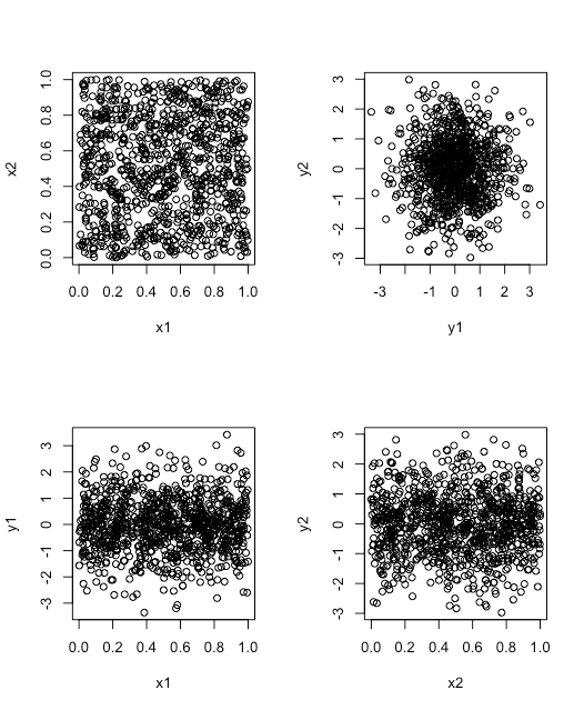
test_script.R. The scatterplot in the upper left uses two vectors drawn at random from a uniform distribution. The scatterplot in the upper right uses two vectors drawn at random from a normal distribution. Each of the scatterplots in the bottom row use two vectors, one drawn at random from a uniform distribution and one drawn at random from a normal distribution. (Copyright; author via source)Loading a Data File and Saving a Data File
Although creating a small vector, data frame, matrix, array, or list is easy, creating one with hundreds of elements or creating dozens of individual data objects is tedious at best; thus, the ability to load data saved during an earlier session, or the ability to read in a spreadsheet file is helpful.
To read in a spreadsheet file saved in .csv format (comma separated values), we use R's read.csv() function, which takes the general form
read.csv(file)
where file provides the absolute path to the file. This is easiest to manage if you navigate to the folder where your .csv file is stored using RStudio's file pane and then set it as the working directory by clicking on More and selecting Set As Working Directory. Download the file "element_data.csv" using this link and then store the file in a folder on your computer. Navigate to this folder and set it as your working directory. Enter the following line of code
elements = read.csv(file = "element_data.csv")
to read the file's data into a data frame named elements . To view the data frame's structure we use the head() function to display the first six rows of data.
head(elements)
name symbol at_no at_wt mp bp phase electronegativity electron_affinity
1 Hydrogen H 1 1.007940 14.01 20.28 Gas 2.20 72.8
2 Helium He 2 4.002602 NA 4.22 Gas NA 0.0
3 Lithium Li 3 6.941000 453.69 1615.15 Solid 0.98 59.6
4 Beryllium Be 4 9.012182 1560.15 2743.15 Solid 1.57 0.0
5 Boron B 5 10.811000 2348.15 4273.15 Solid 2.04 26.7
6 Carbon C 6 12.010700 3823.15 4300.15 Solid 2.55 153.9
block group period at_radius covalent_radius
1 s 1 1 5.30e-11 3.70e-11
2 p 18 1 3.10e-11 3.20e-11
3 s 1 2 1.67e-10 1.34e-10
4 s 2 2 1.12e-10 9.00e-11
5 p 13 2 8.70e-11 8.20e-11
6 p 14 2 6.70e-11 7.70e-11
Note that cells in the spreadsheet with missing values appear here as NA for not available. The melting points (mp) and boiling points (bp) are in Kelvin, and the electron affinities are in kJ/mol.
You can save to your working directory the contents of data frame by using the write.csv() function; thus, we can save a copy of the data in elements using the following line of code
write.csv(elements, file = "element_data_copy.csv")
Another way to save multiple objects is to use the save() function to create an .RData file. For example, to save the vectors v00, v01, and v02 to a file with the name vectors.RData, enter
save(v00, v01, v02, file = "vectors.RData")
To read in the objects in an .RData file, navigate to the folder that contains the file, click on the file's name and RStudio will ask if you wish to load the file into your session.
Using Packages of Functions
The base installation of R provides many useful functions for working with data. The advantage of these functions is that they work (always a plus) and they are stable (which means they will continue to work even as R is updated to new versions). For the most part, we will rely on R’s built in functions for these two reasons. When we need capabilities that are not part of R’s base installation, then we must write our own functions or use packages of functions written by others.
To install a package of functions, click on the Packages tab in the Files, Plots, Packages, Help & Viewer pane. Click on the button labeled Install, enter the name of the package you wish to install, and click on Install to complete the installation. You only need to install a package once.
To use a package that is not part of R’s base installation, you need to bring it into your current session, which you do with the command library(name of package) or by clicking on the checkbox next to the name of the package in the list of your installed packages. Once you have loaded the package into your session, it remains available to you until you quit RStudio.
Managing Your Environment
One nice feature of RStudio is that the Environment Panel provides a list of the objects you create. If your environment becomes too cluttered, you can delete items by switching to the Grid view, clicking on the check-box next to the object(s) you wish to delete, and then clicking on the broom icon. You can remove all items from the List view by simply clicking on the broom icon.
Getting Help
There are extensive help files for R's functions that you can search for using the Help Panel or by using the help() command. A help file shows you the command’s proper syntax, including the types of values you can pass to the command and their default values, if any—more details on this later—and provides you with some examples of how the command is used. R's help files can be difficult to parse at times; you may find it more helpful to simply use a search engine to look for information about "how to use <command> in R." Another good source for finding help with R is stackoverflow.