2.6: Viscosity

Last updated
Save as PDF

Page ID: 55849

\( \newcommand{\vecs}[1]{\overset { \scriptstyle \rightharpoonup} {\mathbf{#1}} } \) \( \newcommand{\vecd}[1]{\overset{-\!-\!\rightharpoonup}{\vphantom{a}\smash {#1}}} \)\(\newcommand{\id}{\mathrm{id}}\) \( \newcommand{\Span}{\mathrm{span}}\) \( \newcommand{\kernel}{\mathrm{null}\,}\) \( \newcommand{\range}{\mathrm{range}\,}\) \( \newcommand{\RealPart}{\mathrm{Re}}\) \( \newcommand{\ImaginaryPart}{\mathrm{Im}}\) \( \newcommand{\Argument}{\mathrm{Arg}}\) \( \newcommand{\norm}[1]{\| #1 \|}\) \( \newcommand{\inner}[2]{\langle #1, #2 \rangle}\) \( \newcommand{\Span}{\mathrm{span}}\) \(\newcommand{\id}{\mathrm{id}}\) \( \newcommand{\Span}{\mathrm{span}}\) \( \newcommand{\kernel}{\mathrm{null}\,}\) \( \newcommand{\range}{\mathrm{range}\,}\) \( \newcommand{\RealPart}{\mathrm{Re}}\) \( \newcommand{\ImaginaryPart}{\mathrm{Im}}\) \( \newcommand{\Argument}{\mathrm{Arg}}\) \( \newcommand{\norm}[1]{\| #1 \|}\) \( \newcommand{\inner}[2]{\langle #1, #2 \rangle}\) \( \newcommand{\Span}{\mathrm{span}}\)\(\newcommand{\AA}{\unicode[.8,0]{x212B}}\)

Introduction

All liquids have a natural internal resistance to flow termed viscosity. Viscosity is the result of frictional interactions within a given liquid and is commonly expressed in two different ways.

Dynamic Viscosity

The first is dynamic viscosity, also known as absolute viscosity, which measures a fluid’s resistance to flow. In precise terms, dynamic viscosity is the tangential force per unit area necessary to move one plane past another at unit velocity at unit distance apart. As one plane moves past another in a fluid, a velocity gradient is established between the two layers (Figure \(\PageIndex{1}\) ). Viscosity can be thought of as a drag coefficient proportional to this gradient.

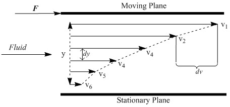
Figure \(\PageIndex{1}\) Fluid dynamics as one plane moves relative to a stationary plane through a liquid. The moving plane has area A and requires force F to overcome the fluid’s internal resistance.

The force necessary to move a plane of area A past another in a fluid is given by Equation \ref{1} where \(V\) is the velocity of the liquid, Y is the separation between planes, and η is the dynamic viscosity.

\[ F = \eta A \frac{V}{Y} \label{1} \]

V/Y also represents the velocity gradient (sometimes referred to as shear rate). Force over area is equal to τ, the shear stress, so the equation simplifies to Equation \ref{2} .

\[ \tau = \eta \frac{V}{Y} \label{2} \]

For situations where V does not vary linearly with the separation between plates, the differential formula based on Newton’s equations is given in Equation \ref{3}.

\[ \tau = \eta \frac{\delta V}{\delta Y} \label{3} \]

Kinematic Viscosity

Kinematic viscosity, the other type of viscosity, requires knowledge of the density, ρ, and is given by Equation \ref{4} , where v is the kinematic viscosity and the \(\eta \) is the dynamic viscosity.

\[ \nu = \frac{\eta }{\rho } \label{4} \]

Units of Viscosity

Viscosity is commonly expressed in Stokes, Poise, Saybolt Universal Seconds, degree Engler, and SI units.

Dynamic Viscosity

The SI units for dynamic (absolute) viscosity is given in units of N·S/m², Pa·S, or kg/(m·s), where N stands for Newton and Pa for Pascal. Poise are metric units expressed as dyne·s/cm² or g/(m·s). They are related to the SI unit by g/(m·s) = 1/10 Pa·S. 100 centipoise, the centipoise (cP) being the most used unit of viscosity, is equal to one Poise. Table \(\PageIndex{1}\) shows the interconversion factors for dynamic viscosity.

Table \(\PageIndex{1}\): The interconversion factors for dynamic viscosity.
Unit	*PaS**	Dyne·s/cm² or g/(m·s) (Poise)	Centipoise (cP)
Pa*S	1	10	1000
Dyne·s/cm² or g/(m·s) (Poise)	0.1	1	100
Centipoise (cP)	0.001	0.01	1

Table \(\PageIndex{2}\): Viscosities of common liquids (*at 0% evaporation volume).
Liquid	\(\eta \) (cP)	Temperature (°C)
Water	0.89	25
Water	0.47	60
Milk	2.0	18
Olive Oil	107.5	20
Toothpaste	70,000 - 100,000	18
Ketchup	1000	30
Custard	1,500	85-90
Crude Oil (WTI)*	7	15

Kinematic Viscosity

The CGS unit for kinematic viscosity is the Stoke which is equal to 10^-4m²/s. Dividing by 100 yields the more commonly used centistoke. The SI unit for viscosity is m²/s. The Saybolt Universal second is commonly used in the oilfield for petroleum products represents the time required to efflux 60 milliliters from a Saybolt Universal viscometer at a fixed temperature according to ASTM D-88. The Engler scale is often used in Britain and quantifies the viscosity of a given liquid in comparison to water in an Engler viscometer for 200cm³ of each liquid at a set temperature.

Newtonian versus Non-Newtonian Fluids

One of the invaluable applications of the determination of viscosity is identifying a given liquid as Newtonian or non-Newtonian in nature.

Newtonian liquids are those whose viscosities remain constant for all values of applied shear stress.
Non-Newtonian liquids are those liquids whose viscosities vary with applied shear stress and/or time.

Moreover, non-Newtonian liquids can be further subdivided into classes by their viscous behavior with shear stress:

Pseudoplastic fluids whose viscosity decreases with increasing shear rate
Dilatants in which the viscosity increases with shear rate.
Bingham plastic fluids, which require some force threshold be surpassed to begin to flow and which thereafter flow proportionally to increasing shear stress.

Measuring Viscosity

Viscometers are used to measure viscosity. There are seven different classes of viscometer:

Capillary viscometers.
Orifice viscometers.
High temperature high shear rate viscometers.
Rotational viscometers.
Falling ball viscometers.
Vibrational viscometers.
Ultrasonic Viscometers.

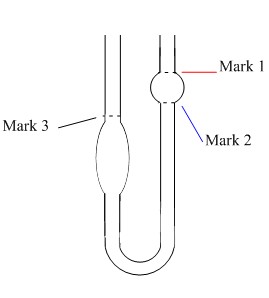
Capillary Viscometers

Capillary viscometers are the most widely used viscometers when working with Newtonian fluids and measure the flow rate through a narrow, usually glass tube. In some capillary viscometers, an external force is required to move the liquid through the capillary; in this case, the pressure difference across the length of the capillary is used to obtain the viscosity coefficient.

Capillary viscometers require a liquid reservoir, a capillary of known dimensions, a pressure controller, a flow meter, and a thermostat be present. These viscometers include, Modified Ostwald viscometers, Suspended-level viscometers, and Reverse-flow viscometers and measure kinematic viscosity.

The equation governing this type of viscometry is the Pouisille law (Equation \ref{5} ), where Q is the overall flowrate, ΔP, the pressure difference, a, the internal radius of the tube, η, the dynamic viscosity, and l the path length of the fluid.

\[ Q\ =\frac{\pi \Delta Pa^{4}}{8\eta l} \label{5} \]

Here, Q is equal to V/t; the volume of the liquid measured over the course of the experiment divided by the time required for it to move through the capillary where V is volume and t is time.

For gravity-type capillary viscometers, those relying on gravity to move the liquid through the tube rather than an applied force, Equation \ref{6} is used to find viscosity, obtained by substituting the relation Equation \ref{5} with the experimental values, where P is pressure, ρ is density, g is the gravitational constant, and h is the height of the column.

\[ \eta \ =\frac{\pi gha^{4}}{8lV} \rho t \label{6} \]

An example of a capillary viscometer (Ostwald viscometer) is shown in Figure \(\PageIndex{2}\).

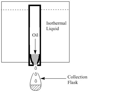
Figure \(\PageIndex{2}\) The capillary, submerged in an isothermal bath, is filled until the liquid lies at Mark 3. The liquid is then drawn up through the opposite side of the tube. The time it takes for the liquid to travel from Mark 2 to Mark 1 is used to compute the viscosity.

Orifice Viscometers

Commonly found in the oil industry, orifice viscometers consist of a reservoir, an orifice, and a receiver. These viscometers report viscosity in units of efflux time as the measurement consists of measuring the time it takes for a given liquid to travel from the orifice to the receiver. These instruments are not accurate as the set-up does not ensure that the pressure on the liquid remains constant and there is energy lost to friction at the orifice. The most common types of these viscometer include Redwood, Engler, Saybolt, and Ford cup viscometers. A Saybolt viscometer is represented in Figure \(\PageIndex{3}\).

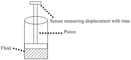
Figure \(\PageIndex{3}\) The time it takes for a 60 mL collection flask to fill is used to determine the viscosity in Saybolt units.

High Temperature, High Shear Rate Viscometers

These viscometers, also known as cylinder-piston type viscometers are employed when viscosities above 1000 poise, need to be determined, especially of non-Newtonian fluids. In a typical set-up, fluid in a cylindrical reservoir is displaced by a piston. As the pressure varies, this type of viscometry is well-suited for determining the viscosities over varying shear rates, ideal for characterizing fluids whose primary environment is a high temperature, high shear rate environment, e.g., motor oil. A typical cylinder-piston type viscometer is shown in Figure \(\PageIndex{4}\).

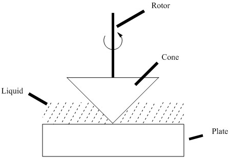
Figure \(\PageIndex{4}\) A typical cylinder-piston type viscometer.

Rotational Viscometers

Well-suited for non-Newtonian fluids, rotational viscometers measure the rate at which a solid rotates in a viscous medium. Since the rate of rotation is controlled, the amount of force necessary to spin the solid can be used to calculate the viscosity. They are advantageous in that a wide range of shear stresses and temperatures and be sampled across. Common rotational viscometers include: the coaxial-cylinder viscometer, cone and plate viscometer, and coni-cylinder viscometer. A cone and plate viscometer is shown in Figure \(\PageIndex{5}\).

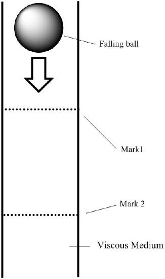
Figure \(\PageIndex{5}\) A cone is spun by a rotor in a liquid paste along a plate. The response of the rotation of the cone is measured, thereby determining viscosity.

Falling Ball Viscometer

This type of viscometer relies on the terminal velocity achieved by a balling falling through the viscous liquid whose viscosity is being measured. A sphere is the simplest object to be used because its velocity can be determined by rearranging Stokes’ law Equation \ref{7} to Equation \ref{8} , where r is the sphere’s radius, η the dynamic viscosity, v the terminal velocity of the sphere, σ the density of the sphere, ρ the density of the liquid, and g the gravitational constant

\[ 6\pi r\eta v\ =\ \frac{4}{3} \pi r^{3} (\sigma - \rho)g \label{7} \]

\[ \eta\ =\frac{\frac{4}{3} \pi r^{2}(\sigma - \rho)g}{6\pi v} \label{8} \]

A typical falling ball viscometric apparatus is shown in Figure \(\PageIndex{6}\).

Figure \(\PageIndex{6}\) The time taken for the falling ball to pass from mark 1 to mark 2 is used to obtain viscosity measurements.

Vibrational Viscometers

ften used in industry, these viscometers are attached to fluid production processes where a constant viscosity quality of the product is desired. Viscosity is measured by the damping of an electrochemical resonator immersed in the liquid to be tested. The resonator is either a cantilever, oscillating beam, or a tuning fork. The power needed to keep the oscillator oscillating at a given frequency, the decay time after stopping the oscillation, or by observing the difference when waveforms are varied are respective ways in which this type of viscometer works. A typical vibrational viscometer is shown in Figure \(\PageIndex{7}\).

Figure \(\PageIndex{7}\) A resonator produces vibrations in the liquid whose viscosity is to be tested. An external sensor detects the vibrations with time, characterizing the material’s viscosity in realtime.

Ultrasonic Viscometers

This type of viscometer is most like vibrational viscometers in that it is obtaining viscosity information by exposing a liquid to an oscillating system. These measurements are continuous and instantaneous. Both ultrasonic and vibrational viscometers are commonly found on liquid production lines and constantly monitor the viscosity.