2.2: Molecular Weight Determination
- Page ID
- 55839

Solution Molecular Weight of Small Molecules
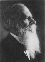
The cryoscopic method was formally introduced in the 1880’s when François-Marie Raoult published how solutes depressed the freezing points of various solvents such as benzene, water, and formic acid. He concluded from his experimentation “if one molecule of a substance can be dissolved in one-hundred molecules of any given solvent then the solvent temperature is lowered by a specific temperature increment”. Based on Raoult’s research, Ernst Otto Beckmann invented the Beckmann thermometer and the associated freezing - point apparatus, which was a significant improvement in measuring freezing - point depression values for a pure solvent. The simplicity, ease, and accuracy of this apparatus has allowed it to remain as a current standard with few modifications for molecular weight determination of unknown compounds.

The historical significance of Raoult and Beckmann’s research, among many other investigators, has revolutionized a physical chemistry technique that is currently applied to a vast range of disciplines from food science to petroleum fluids. For example, measured cryoscopic molecular weights of crude oil are used to predict the viscosity and surface tension for necessary fluid flow calculations in pipeline.
Freezing Point Depression
Freezing point depression is a colligative property in which the freezing temperature of a pure solvent decreases in proportion to the number of solute molecules dissolved in the solvent. The known mass of the added solute and the freezing point of the pure solvent information permit an accurate calculation of the molecular weight of the solute.
In Equation \ref{1} the freezing point depression of a non-ionic solution is described. Where ∆Tf is the change in the initial and final temperature of the pure solvent, Kf is the freezing point depression constant for the pure solvent, and m (moles solute/kg solvent) is the molality of the solution.
\[\Delta T _ { f } = K _ { f } m \label{1} \]
For an ionic solution shown in Figure \(\PageIndex{2}\), the dissociation particles must be accounted for with the number of solute particles per formula unit, \(i\) (the van’t Hoff factor).
\[\Delta T _ { f } = K _ { f } m i\ \label{2} \]
Cryoscopic Procedures
Cryoscopic Apparatus
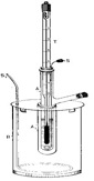
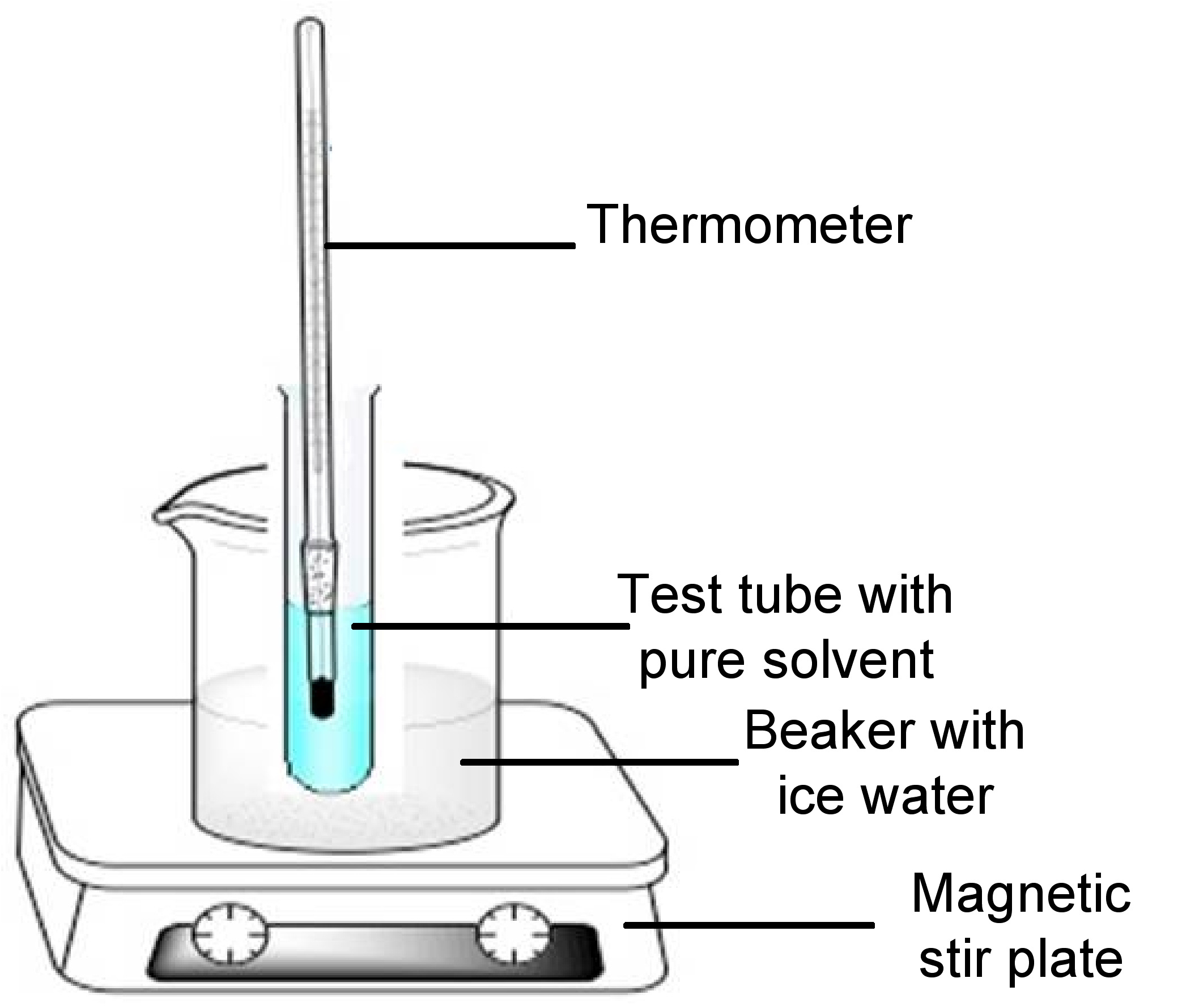
For cryoscopy, the apparatus to measure freezing point depression of a pure solvent may be representative of the Beckmann apparatus previously shown in Figure \(\PageIndex{3}\). The apparatus consists of a test tube containing the solute dissolved in a pure solvent, stir bar or magnetic wire and closed with a rubber stopper encasing a mercury thermometer. The test tube component is immersed in an ice-water bath in a beaker. An example of the apparatus is shown in Figure \(\PageIndex{4}\). The rubber stopper and stir bar/wire stirrer are not shown in the figure.
Sample and Solvent Selection
The cryoscopic method may be used for a wide range of samples with various degrees of polarity. The solute and solvent selection should follow the premise of like dissolved like or in terms of Raoult’s principle of the dissolution of one molecule of solute in one-hundred molecules of a solvent. The most common solvents such as benzene are generally selected because it is unreactive, volatile, and miscible with many compounds.Table \(\PageIndex{1}\) shows the cryoscopic constants (Kf) for the common solvents used for cryoscopy. A complete list of Kf values are available in Knovel Critical Tables.
| Compound | Kf |
|---|---|
| Acetic Acid | 3.90 |
| Benzene | 5.12 |
| Camphor | 39.7 |
| Carbon disulfide | 3.8 |
| Carbon tetrachloride | 30 |
| Chloroform | 4.68 |
| Cyclohexane | 20.2 |
| Ethanol | 1.99 |
| Naphthalene | 6.8 |
| Phenol | 7.27 |
| Water | 1.86 |
Cryoscopic Method
The detailed information about the procedure used for cryoscopy is shown below:
Allow the solution to stir continuously to avoid supercooling
- Weigh (15 to 20 grams) of the pure solvent in a test tube and record the measured weight value of the pure solvent.
- Place a stir bar or wire stirrer in the test tube and close with a rubber stopper that has a hole to encase a mercury thermometer.
- Place a mercury thermometer in the rubber stopper hole.
- Immerse the test tube apparatus in an ice-water bath.
- Allow the solvent to stir continuously and equilibrate to a few degrees below the freezing point of the solvent.
- Record the temperature at which the solvent reaches the freezing point, which remains at a constant temperature reading.
- Repeat the freezing point data collection for at least two more measurements without a difference less than 0.5 °C between the measurements.
- Weigh a quantity of the solute for investigation and record the measured value.
- Add the weighed solute to the test tube containing the pure solvent.
- Re - close the test tube with a rubber stopper encasing a mercury thermometer.
- Re-immerse the test tube in an ice water bath and allow the mixture to stir to fully dissolve the solute in the pure solvent.
- Measure the freezing point and record the temperature value.
The observed freezing point of the solution is when the temperature reading remains constant.
Sample calculation to determine molecular weight
Sample Data Set
Table \(\PageIndex{2}\) represents an example of a data set collection for cryoscopy.
| Parameter | Trial 1 | Trial 2 | Trial 3 | Avg. |
|---|---|---|---|---|
| Mass of cyclohexane (g) | 9.05 | 9.00 | 9.04 | 9.03 |
| Mass of unknown solute (g) | 0.4000 | 0.41010 | 0.4050 | 0.4050 |
| Freezing point of cyclohexane (°C) | 6.5°C | 6.5°C | 6.5°C | 6.5°C |
| Freezing point of cyclohexane mixed with unknown solute (°C) | 4.2°C | 4.3°C | 4.2°C | 4.2°C |
Calculation of molecular weight using the freezing point depression equation
Calculate the freezing point (Fpt) depression of the solution (TΔf) from Equation \ref{3}
\[T \Delta _{f} =\ (Fpt\ of\ pure\ solvent)\ -\ (Fpt\ of\ solution)\ \label{3} \]
\[T \Delta_{f} = \ 6.5^{\circ}C-4.2^{\circ}C \nonumber \]
\[T \Delta_{f} =\ 2.3^{\circ} \nonumber \]
Calculate the molal concentration, m, of the solution using the freezing point depression and Kf (see \label{4})
\[ T \Delta_{f} = K_{f}m\ \label{4} \]
\[m = (2.3^{\circ}C)/(20.2^{\circ}C/molal) \nonumber \]
\[m = 0.113 molal \nonumber \]
\[m = g(solute)/kg(solvent) \nonumber \]
Calculate the MW of the unknown sample.
i = 1 for covalent compounds in \ref{2}
\[M_{W} =\frac{K_{f}(g\ solute)}{\Delta T_{f} (kg solvent)} \nonumber \]
\[M_{W} = \frac{20.2^{\circ}C*kg/moles \times 0.405\ g}{2.3^{\circ}C \times 0.00903\ kg} \nonumber \]
\[M_{W} =\ 393\ g/mol \nonumber \]
Problems
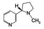
1. Nicotine (Figure \(\PageIndex{5}\) is an extracted pale yellow oil from tobacco leaves that dissolves in water at temperatures less than 60°C. What is the molality of nicotine in an aqueous solution that begins to freeze at -0.445°C? See Table \(\PageIndex{1}\) for Kf values.
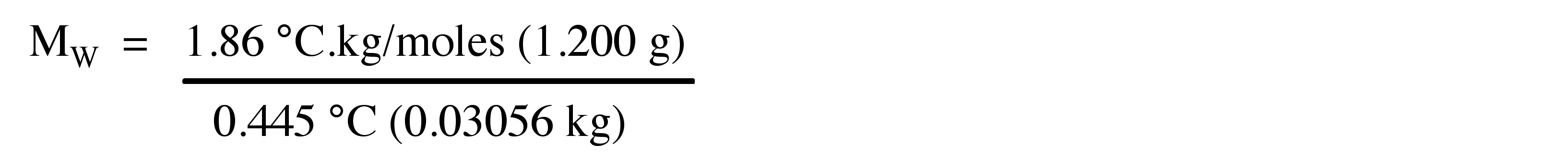
2. If the solution used in Problem 1 is obtained by dissolving 1.200 g of nicotine in 30.56 g of water, what is the molar mass of nicotine?
3. What would be the freezing point depression when 0.500 molal of Ca(NO3)2 is dissolved in 60 g of water?
4. Calculate the number of weighted grams of Ca(NO3)2 added to the 60 g of water to achieve the freezing point depression from Problem 3.
Answers
1.


2.


3.


4.


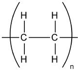
Molecular Weight of Polymers
Knowledge of the molecular weight of polymers is very important because the physical properties of macromolecules are affected by their molecular weight. For example, shown in Figure \(\PageIndex{6}\) the interrelation between molecular weight and strength for a typical polymer. Dependence of mechanical strength on polymer molecular weight. Adapted from G. Odian, Principles of Polymerization, 4th edition, Willey-Interscience, New York (2004).

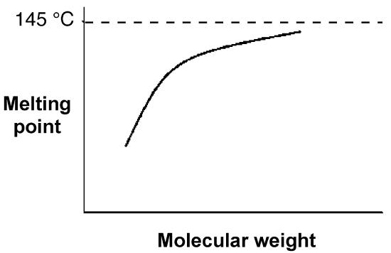
The melting point of polymers are also slightly depend on their molecular weight. Figure \(\PageIndex{7}\) shows relationship between molecular weight and melting temperatures of polyethylene (Figure \(\PageIndex{8}\) ) Most linear polyethylenes have melting temperatures near 140 °C. The approach to the theoretical asymptote, that is a line whose distance to a given curve tends to zero, indicative that a theoretical polyethylene of infinite molecular weight (i.e., M = ∞) would have a melting point of 145 °C.
The molecular weight-melting temperature relationship for the alkane series. Adapted from L. H. Sperling, Introduction to physical polymer science, 4th edition, Wiley-Interscience, New York (2005).
There are several ways to calculate molecular weight of polymers like number average of molecular weight, weight average of molecular weight, Z-average molecular weight, viscosity average molecular weight, and distribution of molecular weight.
Molecular Weight Calculations
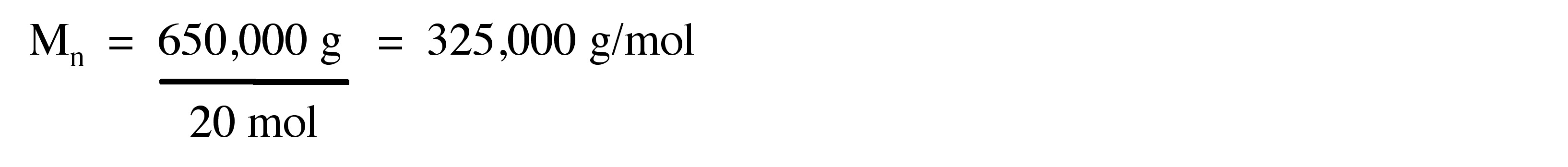
Number average of molecular weight (Mn)
Number average of molecular weight is measured to determine number of particles. Number average of molecular weight is the total weight of polymer, \ref{5}, divided by the number of polymer molecules, \ref{6} . The number average molecular weight (Mn) is given by \ref{7} , where Mi is molecular weight of a molecule of oligomer n, and Ni is number of molecules of that molecular weight.
\[ Total\ weight =\ \Sigma _{i=1} ^{∞} M_{i} N_{i} \label{5} \]
\[ Total\ number = \ \Sigma _{i=1} ^{∞} N _{i} \label{6} \]
\[ M_{n} =\frac{ \Sigma _{i=1} ^{∞} M_{i} N_{i}}{\Sigma _{i=1} ^{∞} N _{i}} \label{7} \]
Consider a polymer sample comprising of 5 moles of polymer molecules having molecular weight of 40.000 g/mol and 15 moles of polymer molecules having molecular weight of 30.000 g/mol.


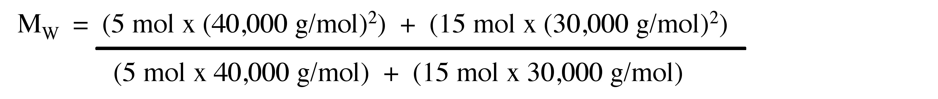
Weight average of molecular weight (MW)
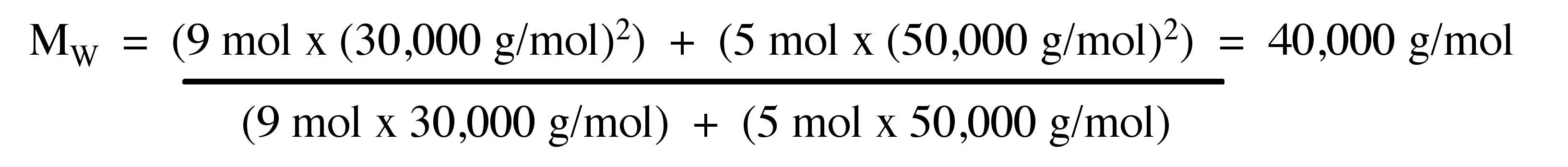
Weight average of molecular weight (MW) is measured to determine the mass of particles. MW defined as \ref{8} , where Mi is molecular weight of oligomer n, and Ni is number of molecules of that molecular weight.
\[ M_{W} =\frac{\Sigma _{i=1} ^{∞} N_{i} (M_{i})^{2}}{\Sigma _{i=1} ^{∞} N_{i} M_{i}} \label{8} \]
Example:
Consider the polymer described in the previous problem.

Calculate the MW for a polymer sample comprising of 9 moles of polymer molecules having molecular weight of 30.000 g/mol and 5 moles of polymer molecules having molecular weight of 50.000 g/mol.
Answer:
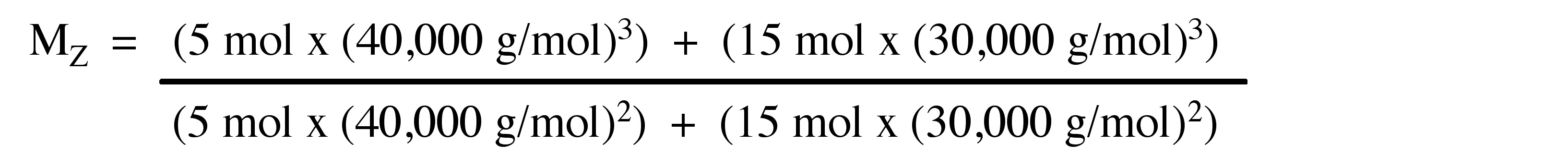
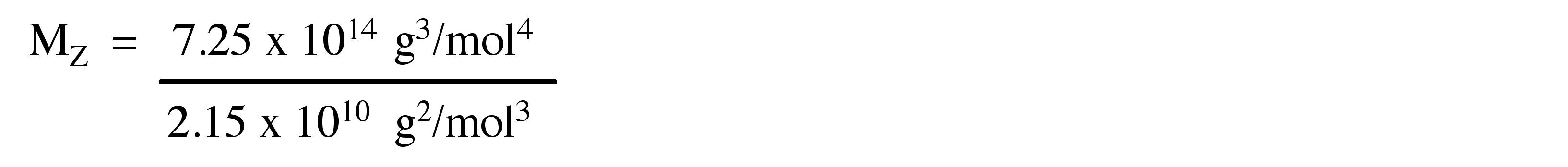
Z-average molecular weight (MZ)
The Z-average molecular weight (Mz) is measured in some sedimentation equilibrium experiments. Mz isn’t common technique for molecular weight of polymers. The molar mass depends on size and mass of the molecules. The ultra centrifugation techniques employ to determine Mz. Mz emphasizes large particles and it defines the EQ, where Mi is molecular weight and Ni is number of molecules.
\[ M_{W} =\frac{\Sigma N_{i} M_{i}^{3}}{\Sigma N_{i} M{i}^{2}} \nonumber \]
Consider the polymer described in the previous problem.

Viscosity average molecular weight (MV)
One of the ways to measure the average molecular weight of polymers is viscosity of solution. Viscosity of a polymer depend on concentration and molecular weight of polymers. Viscosity techniques is common since it is experimentally simple. Viscosity average molecular weight defines as \ref{9} , where Mi is molecular weight and Ni is number of molecules, a is a constant which depend on the polymer-solvent in the viscosity experiments. When a is equal 1, Mv is equal to the weight average molecular weight, if it isn’t equal 1 it is between weight average molecular weight and the number average molecular weight.
\[(\frac{\Sigma N_{i} M_{i} ^{1+a}}{\Sigma N_{i} M_{i}})^{\frac{1}{2}} \label{9} \]
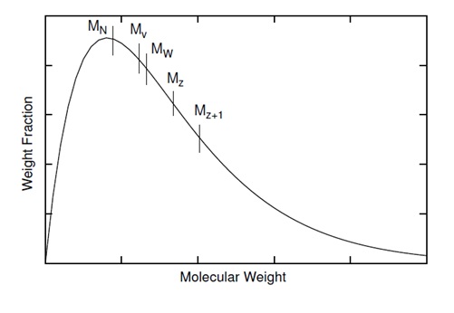
Distribution of molecular weight
Molecular weight distribution is one of the important characteristic of polymer because it affects polymer properties. A typical molecular distribution of polymers show in \(\PageIndex{6}\). There are various molecular weights in the range of curve. The distribution of sizes in a polymer sample isn't totally defined by its central tendency. The width and shape of distribution must be known. It is always true that the various range molecular weight is \ref{10} . The equality is occurring when all polymer in the sample have the same molecular weight.
\[ M_{N} \geq M_{V} \geq M_{W} \geq M_{Z} \geq M_{Z+1} \label{10} \]
Molecular weight analysis of polymers
Gel permeation chromatography (GPC)
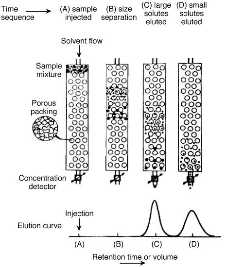
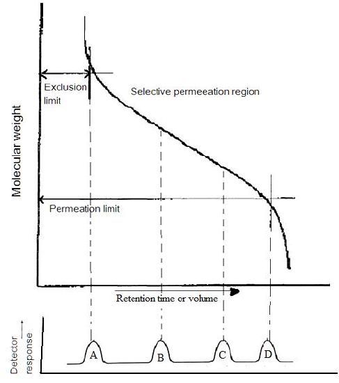
Gel permeation chromatography is also called size exclusion chromatography. It is widely used method to determine high molecular weight distribution. In this technique, substances separate according to their molecule size. Firstly, large molecules begin to elute then smaller molecules are eluted Figure \(\PageIndex{7}\). The sample is injected into the mobile phase then the mobile phase enters into the columns. Retention time is the length of time that a particular fraction remains in the column. As shown in Figure \(\PageIndex{7}\), while the mobile phase passes through the porous particles, the area between large molecules and small molecules is getting increase. GPC gives a full molecular distribution, but its cost is high.

According to basic theory of GPC, the basic quantity measured in chromatography is the retention volume, \ref{11}, where V0 is mobile phase volume and Vp is the volume of a stationary phase. K is a distribution coefficient related to the size and types of the molecules.
\[V_{e} = V_{0} + V_{p} K \label{11} \]
The essential features of gel permeation chromatography are shown in Figure \(\PageIndex{8}\). Solvent leaves the solvent supply, then solvent is pumped through a filter. The desired amount of flow through the sample column is adjusted by sample control valves and the reference flow is adjusted that the flow through the reference and flow through the sample column reach the detector in common front. The reference column is used to remove any slight impurities in the solvent. In order to determine the amount of sample, a detector is located at the end of the column. Also, detectors may be used to continuously verify the molecular weight of species eluting from the column. The flow of solvent volume is as well monitored to provide a means of characterizing the molecular size of the eluting species.

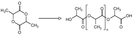
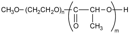
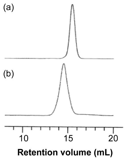
As an example, consider the block copolymer of ethylene glycol (PEG, Figure \(\PageIndex{9}\) ) and poly(lactide) (PLA, Figure \(\PageIndex{10}\) ), i.e., Figure \(\PageIndex{11}\). In the first step starting with a sample of PEG with a Mn of 5,700 g/mol. After polymerization, the molecular weight increased because of the progress of lactide polymerization initiated from end of PEG chain. Varying composition of PEG-PLA shown in Table \(\PageIndex{3}\) can be detected by GPC (Figure \(\PageIndex{12}\) ).
| Polymer | Mn of PEG | Mw/Mn of PEG | Mn of PLA | Mw/Mn of block copolymer | Weight ratio of PLA to PEG |
| PEG-PLA (41-12) | 4100 | 1.05 | 1200 | 1.05 | 0.29 |
| PEG-PLA (60-30) | 6000 | 1.03 | 3000 | 1.08 | 0.50 |
| PEG-PLA (57-54) | 5700 | 1.03 | 5400 | 1.08 | 0.95 |
| PEG-PLA (61-78) | 6100 | 1.03 | 7800 | 1.11 | 1.28 |
Light-scattering
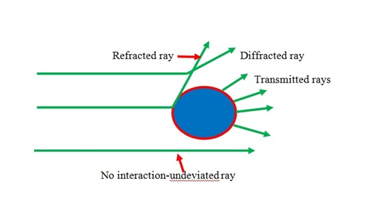
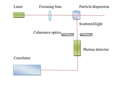
One of the most used methods to characterize the molecular weight is light scattering method. When polarizable particles are placed in the oscillating electric field of a beam of light, the light scattering occurs. Light scattering method depends on the light, when the light is passing through polymer solution, it is measure by loses energy because of absorption, conversion to heat and scattering. The intensity of scattered light relies on the concentration, size and polarizability that is proportionality constant which depends on the molecular weight. Figure \(\PageIndex{13}\) shows light scattering off a particle in solution.
A schematic laser light-scattering is shown in Figure \(\PageIndex{14}\). A major problem of light scattering is to prepare perfectly clear solutions. This problem is usually accomplished by ultra-centrifugation. A solution should be as possible as clear and dust free to determine absolute molecular weight of polymer. The advantages of this method, it doesn’t need calibration to obtain absolute molecular weight and it can give information about shape and Mw information. Also, it can be performed rapidly with less amount of sample and absolute determinations of the molecular weight can be measured. The weaknesses of the method is high price and most times it requires difficult clarification of the solutions.
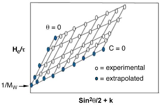
The weight average molecular weight value of scattering polymers in solution related to their light scattering properties that define by \ref{12} , where K is the wave vector, that defined by \ref{13} . C is solution concentration, R(θ) is the reduced Rayleigh ratio, P(θ) the particle scattering function, θ is the scattering angle, A is the osmotic virial coefficients, where n0 solvent refractive index, λ the light wavelength and Na Avagadro’s number. The particle scattering function is given by \ref{14} , where Rz is the radius of gyration.
\[ KC / R( \theta )\ = \ 1/M_{W} ( P( \theta) \ +\ 2A_{2}C\ +\ 3A_{3}C_{2}\ +\ ...) \label{12} \]
\[ K\ =\ 2 \pi ^{2}n_{0}^{2}(dn/dC)^{2}/N_{a} \lambda ^{2} \label{13} \]
\[ 1/(P(\theta )) \ =\ 1+16 \pi ^{2} n_{0} ^{2} ( R _{z} ^{2} )sin ^{2} ( \theta /2) 3 \lambda ^{2} \label{14} \]
Weight average molecular weight of a polymer is found from extrapolation of data in the form of a Zimm plot ( Figure \(\PageIndex{15}\) ). Experiments are performed at several angles and at least at 4 different concentrations. The straight line extrapolations provides Mw.
X-ray Scattering
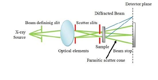
X-rays are a form of electromagnetic wave with wavelengths between 0.001 nm and 0.2 nm. X-ray scattering is particularly used for semicrystalline polymers which includes thermoplastics, thermoplastic elastomers, and liquid crystalline polymers. Two types of X-ray scattering are used for polymer studies:
- Wide-angle X-ray scattering (WAXS) which is used to study orientation of the crystals and the packing of the chains.
- Small-angle X-ray scattering (SAXS) which is used to study the electron density fluctuations that occur over larger distances as a result of structural inhomogeneities.
Schematic representation of X-ray scattering shows in Figure \(\PageIndex{16}\).
At least two SAXS curves are required to determine the molecular weight of a polymer. The SAXS procedure to determine the molecular weight of polymer sample in monomeric or multimeric state solution requires the following conditions.
a. The system should be monodispersed.
b. The solution should be dilute enough to avoid spatial correlation effects.
c. The solution should be isotropic.
d. The polymer should be homogenous.
Osometer
Osmometry is applied to determine number average of molecular weight (Mn). There are two types of osmometer:
- Vapor pressure osmometry (VPO).
- Membrane osmometry.
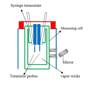
Vapor pressure osmometry measures vapor pressure indirectly by measuring the change in temperature of a polymer solution on dilution by solvent vapor and is generally useful for polymers with Mn below 10,000–40,000 g/mol. When molecular weight is more than that limit, the quantity being measured becomes very small to detect. A typical vapor osmometry shows in the Figure \(\PageIndex{17}\). Vapor pressure is very sensitive because of this reason it is measured indirectly by using thermistors to measure voltage changes caused by changes in temperature.
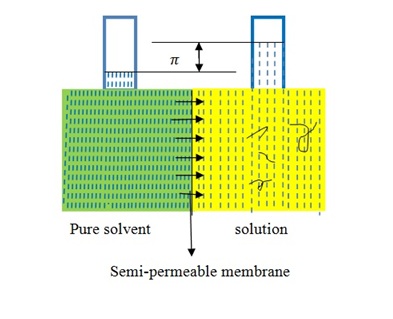
Membrane osmometry is absolute technique to determine Mn(Figure \(\PageIndex{18}\) ). The solvent is separated from the polymer solution with semipermeable membrane that is strongly held between the two chambers. One chamber is sealed by a valve with a transducer attached to a thin stainless steel diaphragm which permits the measurement of pressure in the chamber continuously. Membrane osmometry is useful to determine Mn about 20,000-30,000 g/mol and less than 500,000 g/mol. When Mn of polymer sample more than 500,000 g/mol, the osmotic pressure of polymer solution becomes very small to measure absolute number average of molecular weight. In this technique, there are problems with membrane leakage and symmetry. The advantages of this technique is that it doesn’t require calibration and it gives an absolute value of Mn for polymer samples.
Summary
Properties of polymers depend on their molecular weight. There are different kind of molecular weight and each can be measured by different techniques. The summary of these techniques and molecular weight is shown in the Table \(\PageIndex{4}\).
| Method | Type of Molecular Weight | Range of Application |
| Light Scattering | MW | ∞ |
| Membrane Osmometry | Mn | 104 -106 |
| Vapor Phase Osmometry | Mn | 40,000 |
| X-ray scattering | Mw, n, z | 102 |
Size Exclusion Chromatography and its Application in Polymer Science
Size exclusion chromatography (SEC) is a useful technique that is specifically applicable to high-molecular-weight species, such as polymer. It is a method to sort molecules according to their sizes in solution. The sample solution is injected into the column, which is filled with rigid, porous, materials, and is carried by the solvent through the packed column. The sizes of molecules are determined by the pore size of the packing particle in the column within which the separation occurs.
For polymeric materials, the molecular weight (Mw) or molecular size plays a key role in determining the mechanical, bulk, and solution properties of materials. It is known that the sizes of polymeric molecules depend on their molecular weights, side chain configurations, molecular interaction, and so on. For example, the exclusion volume of polymers with rigid side group is larger than those with soft long side chains. Therefore, in order to determine the molecular weight and molecular weight distribution of a polymer, one of the most widely applied methods is gel-permeation chromatography.
Gel permeation chromatography (GPC) is a term used for when the separation technique size exclusion chromatography (SEC) is applied to polymers.
The primary purpose and use of the SEC technique is to provide molecular weight distribution information about a particular polymeric material. Typically, in about 30 minutes using standard SEC, the complete molecular weight distribution of a polymer as well as all the statistical information of the distribution can be determined. Thus, SEC has been considered as a technique essentially supplanting classical molecular weight techniques. To apply this powerful technique, there is some basic work that needs to be done before its use. The selection of an appropriate solvent and the column, as well as the experimental conditions, are important for proper separation of a sample. Also, it is necessary to have calibration curves in order to determine the relative molecular weight from a given retention volume/time.
It is well known that both the majority of natural and synthetic polymers are polydispersed with respect to molar mass. For synthetic polymers, the more mono-dispersed a polymer can be made, the better the understanding of its inherent properties will be obtained.
Polymer Properties
A polymer is a large molecule (macromolecule) composed of repeating structural units typically connected by covalent chemical bonds. Polymers are common materials that are widely used in our lives. One of the most important features which distinguishes most synthetic polymers from simple molecular compounds is the inability to assign an exact molar mass to a polymer. This is a consequence of the fact that during the polymerization reaction the length of the chain formed is determined by several different events, each of which have different reaction rates. Hence, the product is a mixture of chains of different length due to the random nature of growth. In addition, some polymers are also branched (rather than linear) as a consequence of alternative reaction steps. The molecular weight (Mw) and molecular weight distribution influences many of the properties of polymers:
- Processability - the suitability of the polymer to physical processing.
- Glass-transition temperature - refers to the transformation of a glass-forming liquid into a glass.
- Solution viscosity - measure of the resistance of a fluid which is being deformed by either shear stress or tensile stress.
- Hardness - a measure of how resistant a polymer is to various kinds of permanent shape change when a force is applied.
- Melt viscosity - the rate of extrusion of thermoplastics through an orifice at a prescribed temperature and load.
- Tear strength - a measure of the polymers resistance to tearing.
- Tensile strength - as indicated by the maxima of a stress-strain curve and, in general, is the point when necking occurs upon stretching a sample.
- Stress-crack resistance - the formation of cracks in a polymer caused by relatively low tensile stress and environmental conditions.
- Brittleness - the liability of a polymer to fracture when subjected to stress.
- Impact resistance - the relative susceptibility of polymers to fracture under stresses applied at high speeds.
- Flex life - the number of cycles required to produce a specified failure in a specimen flexed in a prescribed manner.
- Stress relaxation - describes how polymers relieve stress under constant strain.
- Toughness - the resistance to fracture of a polymer when stressed.
- Creep strain - the tendency of a polymer to slowly move or deform permanently under the influence of stresses.
- Drawability - The ability of fiber-forming polymers to undergo several hundred percent permanent deformation, under load, at ambient or elevated temperatures.
- Compression - the result of the subjection of a polymer to compressive stress.
- Fatigue - the failure by repeated stress.
- Tackiness - the property of a polymer being adhesive or gummy to the touch.
- Wear - the erosion of material from the polymer by the action of another surface.
- Gas permeability - the permeability of gas through the polymer.
Consequently, it is important to understand how to determine the molecular weight and molecular weight distribution.
Molecular Weight
Simpler pure compounds contain the same molecular composition for the same species. For example, the molecular weight of any sample of styrene will be the same (104.16 g/mol). In contrast, most polymers are not composed of identical molecules. The molecular weight of a polymer is determined by the chemical structure of the monomer units, the lengths of the chains and the extent to which the chains are interconnected to form branched molecules. Because virtually all polymers are mixtures of many large molecules, we have to resort to averages to describe polymer molecular weight.
The polymers produced in polymerization reactions have lengths which are distributed according to a probability function which is governed by the polymerization reaction. To define a particular polymer weight average, the average molecular weight Mavg is defined by \ref{15} Where Ni is the number of molecules with molecular weight Mi.
\[ M_{avg} \ =\ \frac{\Sigma N_{i} M_{i}^{a}}{\Sigma N_{i} M_{i} ^{a-1}} \label{15} \]
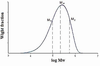
There are several possible ways of reporting polymer molecular weight. Three commonly used molecular weight descriptions are: the number average (Mn), weight average (Mw), and z-average molecular weight (Mz). All of three are applicable to different constant a in \ref{16} and are shown in Figure \(\PageIndex{19}\).
When a = 1, the number average molecular weight, \ref{16} .
\[ M_{n,\ avg} \ =\ \frac{\Sigma N_{i}M_{i}}{\Sigma N_{i}}\ =\ \frac{w}{N} \label{16} \]
When a = 2, the number average molecular weight, \ref{17} .
\[ M_{n,\ avg} \ =\ \frac{\Sigma N_{i}M_{i}^{2}}{\Sigma N_{i}M_{i}}\ =\ \frac{\Sigma N_{i}M_{i}}{w} \label{17} \]
When a = 2, the number average molecular weight, \ref{18} .
\[ M_{n,\ avg} \ =\ \frac{\Sigma N_{i}M_{i}^{3}}{\Sigma N_{i}M_{i}^{2}}\ =\ \frac{\Sigma N_{i}M_{i}^{2}}{\Sigma N_{i}M_{i}} \label{18} \]
Bulk properties weight average molecular weight, Mw is the most useful one, because it fairly accounts for the contributions of different sized chains to the overall behavior of the polymer, and correlates best with most of the physical properties of interest.
There are various methods published to detect these three different primary average molecular weights respectively. For instance, a colligative method, such as osmotic pressure, effectively calculates the number of molecules present and provides a number average molecular weight regardless of their shape or size of polymers. The classical van’t Hoff equation for the osmotic pressure of an ideal, dilute solution is shown in \ref{19} .
\[ \frac{\pi }{c}\ =\ \frac{RT}{M_{n}} \label{19} \]
The weight average molecular weight of a polymer in solution can be determined by either measuring the intensity of light scattered by the solution or studying the sedimentation of the solute in an ultracentrifuge. From light scattering method which is depending on the size rather than the number of molecules, weight average molecular weight is obtained. This work requires concentration fluctuations which are the main source of the light scattered by a polymer solution. The intensity of the light scattering of polymer solution is often expressed by its turbidity τ which is given in Rayleigh’s law in \ref{20} . Where iθ is scattered intensity at only one angle θ, r is the distance from the scattering particle to the detection point, and I0 is the incident intensity.
\[ \tau\ =\ \frac{16\pi i_{\Theta} r^{2}}{3I_{0}(1+cos^{2}\Theta )} \label{20} \]
The intensity scattered by molecules (Ni) of molecular weight (Mi) is proportional to NiMi2. Thus, the total light scattered by all molecules is described in \ref{21} , where c is the total weight of the sample ∑NiMi.
\[ \frac{\pi}{c} ~ \frac{\Sigma N_{i}M_{i}^{2}}{\Sigma N_{i}M_{i}}\ =\ M_{W,\ avg} \label{21} \]
Poly-disperse index (PDI)
The polydispersity index (PDI), is a measure of the distribution of molecular mass in a given polymer sample. As shown in Figure \(\PageIndex{19}\), it is the result of the definitions that Mw ≥ Mn. The equality of Mw and Mn would correspond with a perfectly uniform (monodisperse) sample. The ratio of these average molecular weights is often used as a guide to the dispersity of the chain lengths in a polymer sample. The greater Mw / Mn is, the greater the dispersity is.
The properties of a polymer sample are strongly dependent on the way in which the weights of the individual molecules are distributed about the average. The ratio Mw/Mn gives sufficient information to characterize the distribution when the mathematical form of the distribution curve is known.
Generally, the narrow molecular weight distribution materials are the models for much of work aimed at understanding the materials’ behaviors. For example, polystyrene and its block copolymer polystyrene-b-polyisoprene have quite narrow distribution. As a result, narrow molecular weight distribution materials are a necessary requirement when people study their behavior, such as self-assembly behavior for block copolymer. Nonetheless, there are still lots of questions for scientists to explore the influence of polydispersity. For example, research on self-assembly which is one of the interesting fields in polymer science shows that we cannot throw polydispersity away.
Setup of SEC Equipment
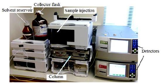
In SEC, sample components migrate through the column at different velocities and elute separately from the column at different times. In liquid chromatography and gas chromatography, as a solute moves along with the carrier fluid, it is at times held back either by surface of the column packing, by stationary phase, or by both. Unlike gas chromatography (GC) and liquid chromatography (LC), molecular size, or more precisely, molecular hydrodynamic volume governs the separation process of SEC, not varied by the type of mobile phase. The smallest molecules are able to penetrate deeply into pores whereas the largest molecules are excluded by the smaller pore sizes. Figure \(\PageIndex{20}\) shows the regular instrumental setup of SEC.
The properties of mobile phase are still important in that it is supposed to be strong affinity to stationary phase and be a good solubility to samples. The purpose of well soluble of sample is to make the polymer be perfect coil suspending in solution. Thus, as a mixture of solutes of different size passes through a column packed with porous particles. As shown in Figure \(\PageIndex{21}\), it clearly depicts the general idea for size separation by SEC. the main setup of SEC emphasizes three concepts: stationary phase (column), mobile phase (solvent) and sample preparation.
Solvent Selection
Solvent selection for SEC involves a number if considerations, such as convenience, sample type, column packing, operating variables, safety, and purity.
For samples concern, the solvents used for mobile phase of SEC are limited to those follows following criteria:
- The solvent must dissolve the sample completely.
- The solvent has different properties with solute in the eluent: typically with solvent refractive index (RI) different from the sample RI by ± 0.05 unit of more, or more than 10% of incident energy for UV detector.
- The solvent must not degrade the sample during use. Otherwise, the viscosity of eluent will gradually increase over times.
- The solvent is not corrosive to any components of the equipment.
Therefore, several solvents are qualified to be solvents such as THF, chlorinated hydrocarbons (chloroform, methylene chloride, dichloroethane, etc), aromatic hydrocarbons (benzene, toluene , trichlorobenzene, etc).
Normally, high purity of solvent (HPLC-grade) is recommended. The reasons are to avoid suspended particulates that may abrade the solvent pumping system or cause plugging of small-particle columns, to avoid impurities that may generate baseline noise, and to avoid impurities that are concentrated due to evaporation of solvent.
Column Selection
Column selection of SEC depends mainly on the desired molecular weight range of separation and the nature of the solvents and samples. Solute molecules should be separated solely by the size of gels without interaction of packing materials. Better column efficiencies and separations can be obtained with small particle packing in columns and high diffusion rates for sample solutes. Furthermore, optimal performance of an SEC packing materials involves high resolution and low column backpressure. Compatible solvent and column must be chosen because, for example, organic solvent is used to swell the organic column packing and used to dissolve and separate the samples.
It is convenient that columns are now usually available from manufacturers regarding the various types of samples. They provide the information such as maximum tolerant flow rates, backpressure tolerances, recommended sample concentration, and injection volumes, etc. Nonetheless, users have to notice a few things upon using columns:
- Vibration and extreme temperatures should be avoided because these will post irreversible damage on columns.
- For aqueous mobile phase, it is unwise to allow the extreme pH solutions staying in the columns for a long period of time.
- The columns should be stored with some neat organic mobile phase, or aqueous mobile phase with pH range 2 - 8 to prevent degradation of packing when not in use.
Sample Preparation
The sample solutions are supposed to be prepared in dilute concentration (less than 2 mg/mL) for several concerns. For polymer samples, samples must be dissolved in the solvent same as used for mobile phase except some special cases. A good solvent can dissolve a sample in any proportion in a range of temperatures. It is a slow process for dissolution because the rate determining step is solvent diffusion into polymers to produce swollen gels. Then, gradual disintegration of gels makes sample-solvent mixture truly become solution. Agitation and warming the mixtures are useful methods to speed up sample preparation.
It is recommended to filter the sample solutions before injecting into columns or storing in sample vials in order to get rid of clogging and excessively high pressure problems. If unfortunately the excessively high pressure or clogging occur due to higher concentration of sample solution, raising the column temperature will reduce the viscosity of the mobile phase, and may be helpful to redissolve the precipitated or adsorbed solutes in the column. Back flushing of the columns should only be used as the last resort.
Analysis of SEC Data
The size exclusion separation mechanism is based on the effective hydrodynamic volume of the molecule, not the molecular weight, and therefore the system must be calibrated using standards of known molecular weight and homogeneous chemical composition. Then, the curve of sample is used to compare with calibration curve and obtain information relative to standards. The further step is required to covert relative molecular weight into absolute molecular weight of a polymer.
Calibration
The purpose of calibration in SEC is to define the relationship between molecular weight and retention volume/time in the chosen permeation range of column set and to calculate the relative molecular weight to standard molecules. There are several calibration methods are commonly employed in modern SEC: direct standard calibration, poly-disperse standard calibration, universal calibration.
The most commonly used calibration method is direct standard calibration. In the direct standard calibration method, narrowly distributed standards of the same polymer being analyzed are used. Normally, narrow-molecular weight standards commercially available are polystyrene (PS). The molecular weight of standards are measured originally by membrane osmometry for number-average molecular weight, and by light scattering for weight-average molecular weight as described above. The retention volume at the peak maximum of each standard is equated with its stated molecular weight.
Relative Mw versus absolute Mw
The molecular weight and molecular weight distribution can be determined from the calibration curves as described above. But as the relationship between molecular weight and size depends on the type of polymer, the calibration curve depends on the polymer used, with the result that true molecular weight can only be obtained when the sample is the same type as calibration standards. As Figure \(\PageIndex{23}\) depicted, large deviations from the true molecular weight occur in the instance of branched samples because the molecular density of these is higher than in the linear chains.

Light-scattering detector is now often used to overcome the limitations of conventional SEC. These signals depend only on concentration, not on molecular weight or polymer size. For instance, for LS detector, \ref{22} applies:
\[LS\ Signal\ =\ K_{LS} \cdot (dn/dc)^{2}\cdot M_{W} \cdot c \label{22} \]
Where KLS is an apparatus-specific sensitivity constant, dn/dc is the refractive index increment and c is concentration. Therefore, accurate molecular weight can be determined while the concentration of the sample is known without calibration curve.
A Practical Example
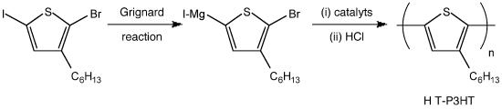
The syntheses of poly(3-hexylthiophene) are well developed during last decade. It is an attractive polymer due to its potential as electronic materials. Due to its excellent charge transport performances and high solubility, several studies discuss its further improvement such as making block copolymer even triblock copolymer. The details are not discussed here. However, the importance of molecular weight and molecular weight distribution is still critical.
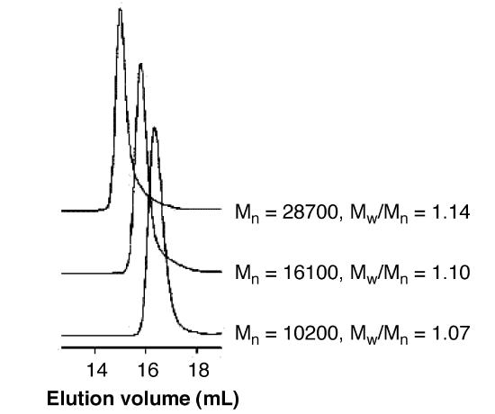
As shown in Figure \(\PageIndex{24}\), they studied the mechanism of chain-growth polymerization and successfully produced low polydispersity P3HT. The figure also demonstrates that the molecule with larger molecular size/ or weight elutes out of the column earlier than those which has smaller molecular weight.
The real molecular weight of P3HT is smaller than the molecular weight relative to polystyrene. In this case, the backbone of P3HT is harder compared with polystyrenes’ backbone because of the position of aromatic groups. It results in less flexibility. We can briefly judge the authentic molecular weight of the synthetic polymer according to its molecular structure.