
1.6: Analysis of Multistage Processes
- Page ID
- 222826

For multistage process, it is recommended to perform kinetic analysis using the following algorithm. Kinetic analysis is performed separately for each of the stages of the process as for a one-stage reaction, and the corresponding kinetic model and kinetic parameters are determined. Then, kinetic analysis is performed for the entire process using the data obtained for the model of each stage. In so doing, the kinetic parameters of each stage are refined. Thus, when the process is studied as a whole, there is already no need to try different kinetic models since they have been chosen for each stage.
However, for most multistage processes, the effects overlap. To separate quasi-one-stage processes, the Peak Separation software can be used. In general case reaction steps are dependent, so the separation procedure is formal. Obtained peaks does not refer to the single reactions and may be used just for the initial approximation of the Arrenius parameters. In the case of the independent reactions separated peaks refer to the single reactions and thus may be used for calculation of the Arrenius parameters.
6.1 Peak Separation Software
In multistage processes with competing or parallel reactions, separate stages, as a rule, overlap, which can lead to considerable errors in the calculated Arrhenius parameters and to an incorrect choice of the scheme of the processes. This in turn will lead to significant errors of the nonlinear regression method because of the nonlinearity of the problem. To solve this problem, the experimental curve is represented by a superposition of separate one-stage processes. This procedure in implemented in the NETZSCH Peak Separation software (Figure 6.1).
The NETZSCH Peak Separation software [13] fits experimental data by a superposition of separate peaks, each of which can be described by one of the following functions:
- Gaussian function,
- Cauchy function,
- pseudo-Voigt function (the sum of the Gaussian and Cauchy functions with corresponding weights),
- Fraser–Suzuki function (the asymmetric Gaussian function),
- Pearson function (monotonic transformation from the Gaussian to the Cauchy function),
- modified Laplace function.
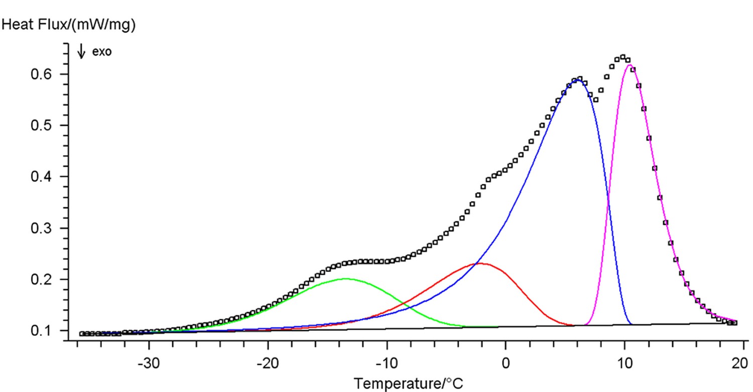
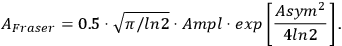
In thermal analysis, chemical reaction steps are described in most cases by the Fraser–Suzuki function (asymmetric Gaussian function). For other processes, e.g., polymer melting, the modified Laplace function must be used. Figure 6.1 shows the decomposition of a multimodal curve with the use of this function and its analytical representation. The Fraser–Suzuki function (asymmetric Gaussian function) and its graphical representation are given below.
\[A_{F \text { raser }}=0.5 \cdot \sqrt{\pi / \ln 2} \cdot A m p l \cdot \exp \left[\frac{A s y m^{2}}{4 \ln 2}\right]\]
The software outputs the following parameters:
- the optimal curve parameters and their standard deviations,
- statistical parameters characterizing the fit quality (correlation coefficient and so on.),
- the initial and simulated curves with the graphs of separate peaks,
- calculated areas under separate peaks and their contribution to the total area under the curve.
6.2 Multiple Step Reaction Analysis as Exemplified by the Carbonization of Oxidized PAN Fiber
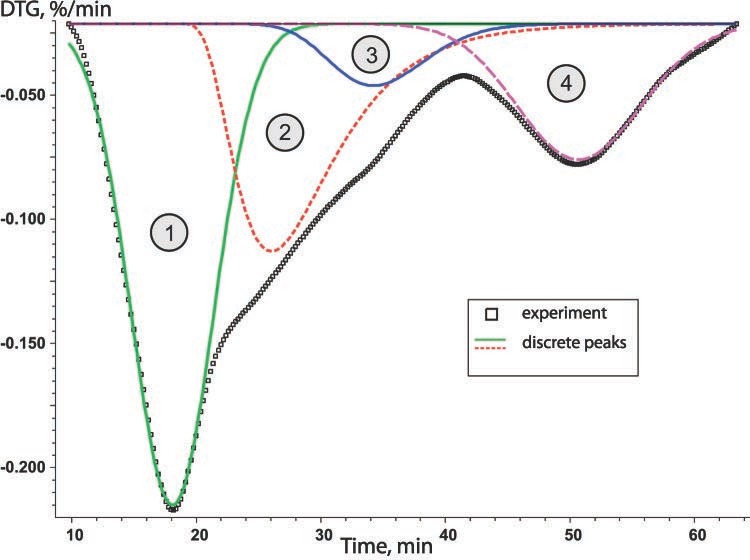
First, multimodal curves are decomposed into separate components and parameters of each process are found by the above procedures, assuming that all processes are quasi-one-stage reactions. Then, the phenomenon is described as a whole. For multiple step processes, the program suggests a list of some schemes of similar transformations, and appropriate schemes are selected from this list. The schemes are presented in Figure 1 of the Appendix. The choice of the corresponding scheme is based on some a priori ideas about the character of stages of the process under consideration.
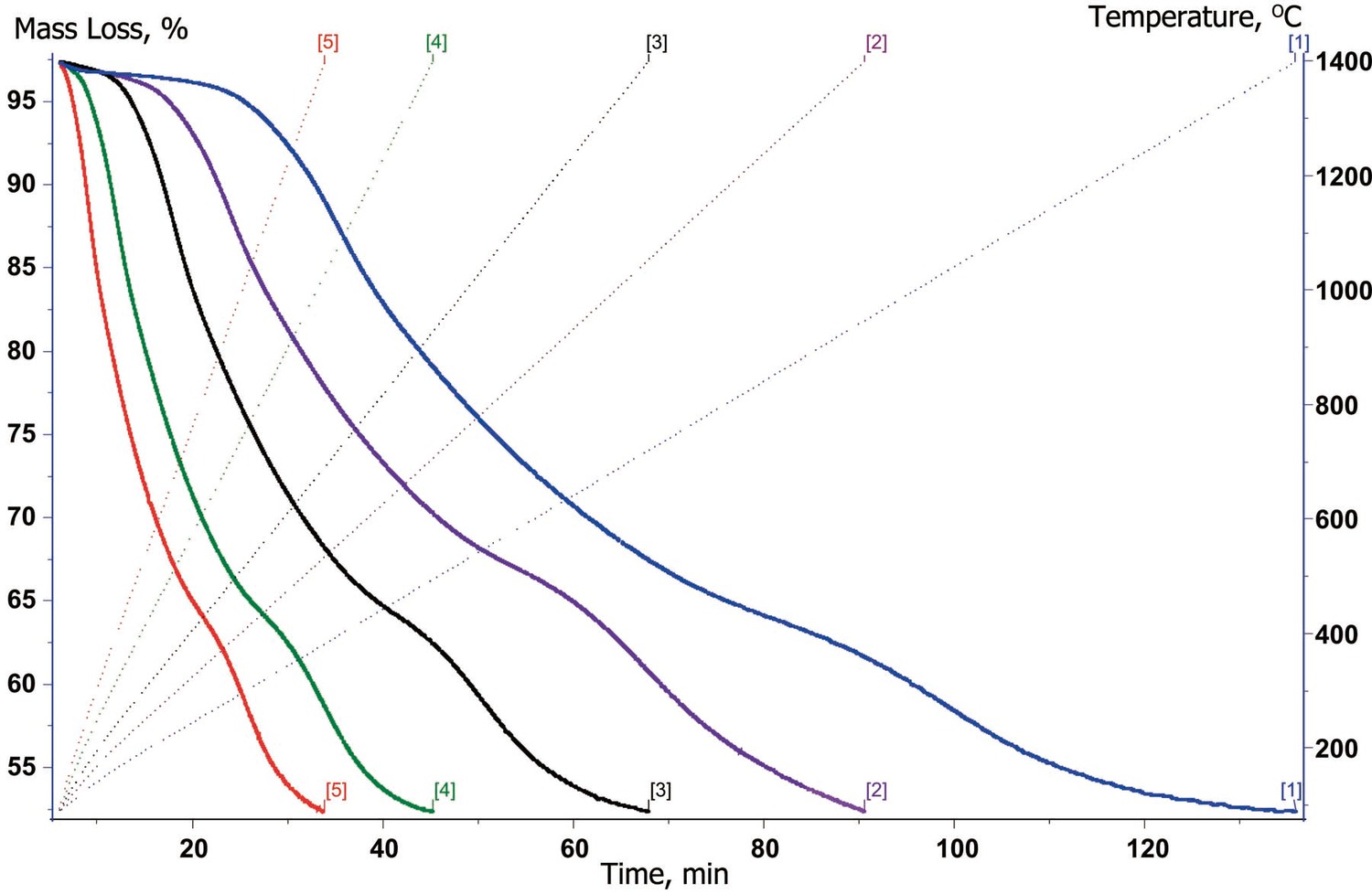
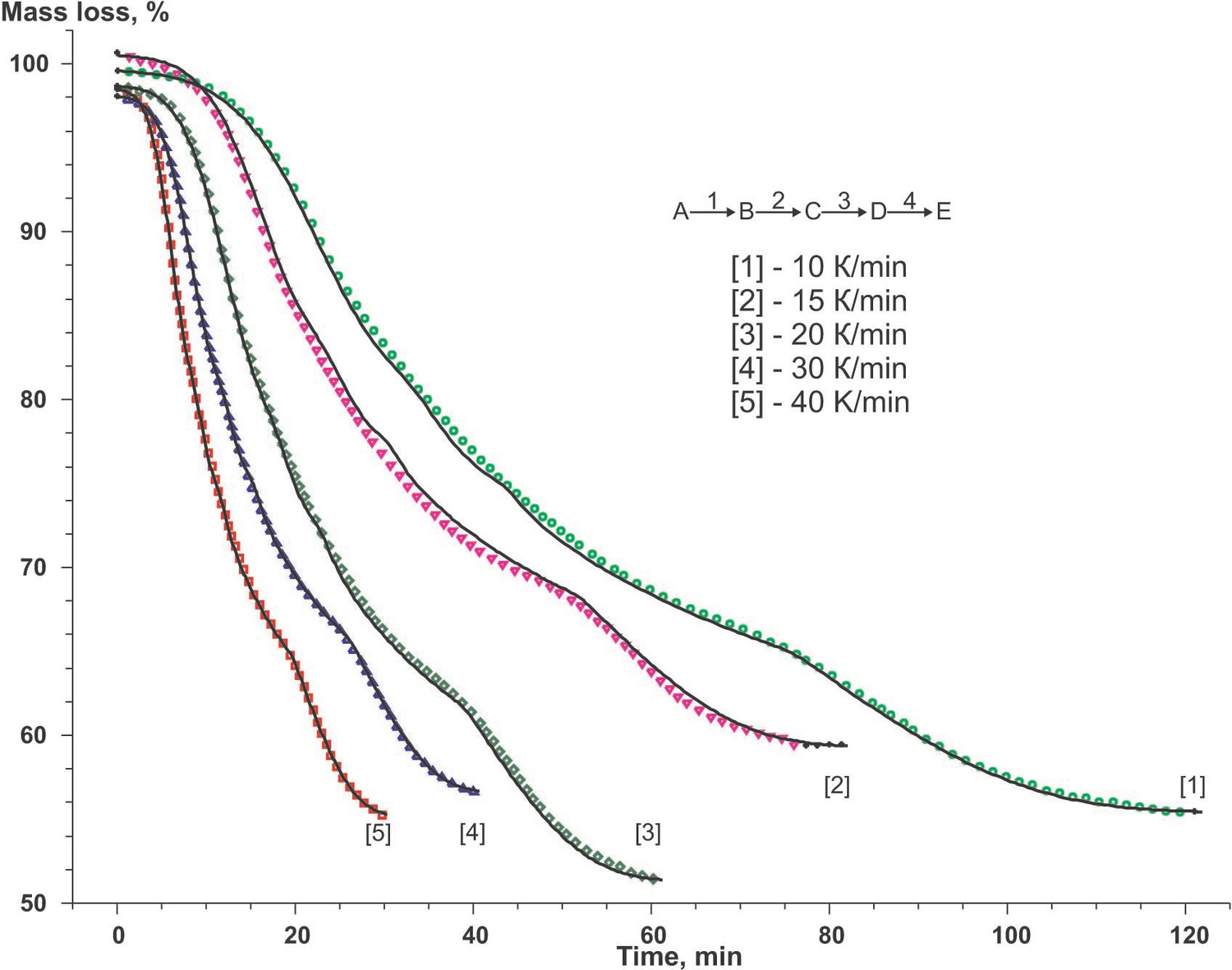
As an example of the kinetic analysis of multistage processes, let us consider the carbonization of oxidized polyacrylonitrile fiber yielding carbon fiber. The results of thermogravimetric analysis are convenient to use as input data (Figure 6.3).
Then, the resulting peaks are sorted on the basis of the number of stage and the inverse kinetic problem is solved. As a result, we obtain the type of model for the given stage and approximate Arrhenius parameters. As a rule, several models of comparable statistical significance satisfy the solution of this problem. If no information is available on the true mechanism of the process, both variants are used for solving the direct kinetic problem.
The estimated parameters and types of models calculated at this step of calculations are listed in Table 6.1, and statistical data of the calculation is presented in Table 6.3. In Table 6.1, the “apparent” activation energy is expressed in kelvins since the notion of mole has no physical meaning for fiber. The Ea/R constant is the temperature coefficient of the reaction rate.
| N | Kinetic model | Ea/R*103K | t•S | log A | t•S | n | t•S |
|---|---|---|---|---|---|---|---|
| 1 | Avrami–Erofeev equation | 25.0 | 0.6 | 14.8 | 0.4 | 0.28 | 0.3 x 10⁻³ |
| 2 | nth order equation | 17.2 | 0.8 | 7.2 | 6.5 | 3.0 | 0.13 |
| 3 | Avrami–Erofeev equation | 41.1 | 2.3 | 16.2 | 1.0 | 0.29 | 0.1 x 10⁻³ |
| 4 | Avrami–Erofeev equation | 54.8 | 1.3 | 16.0 | 0.4 | 0.32 | 3.3 x 10⁻³ |
6.1 Estimated kinetic models and parameters of separate stages of the carbonization process.
| N | Kinetic model | EaR*103K | t•S | log A | t•S | n | t•S |
|---|---|---|---|---|---|---|---|
| 1 | Avrami–Erofeev equation | 26.1 | 0.6 | 15.7 | 0.4 | 0.25 | 4.2*10-3 |
| 2 | nth order equation | 35.5 | 2.1 | 18.8 | 1.2 | 1.98 | 0.14 |
| 3 | Avrami–Erofeev equation | 38.3 | 2.1 | 16.7 | 1.0 | 0.28 | 0.1*10-3 |
| 4 | Avrami–Erofeev equation | 56.8 | 4.7 | 16.8 | 1.6 | 0.19 | 0.1*10-3 |
6.2 Calculated kinetic models and parameters of separate stages of the carbonization process.
| Parameter | Stage 1 | Stage 2 | Stage 3 | Stage 4 |
|---|---|---|---|---|
| Least-squares value | 22.3 | 32.0 | 2.6 | 7.1 |
| Correlation coefficient | 0.9988 | 0.9926 | 0.9956 | 0.9979 |
| Average difference | 2.2 x 10⁻³ | 21.0 x 10⁻³ | 8.6 x 10⁻³ | 14.5 x 10⁻³ |
| Durbin–Watson test value | 2.8 x 10⁻³ | 1.4 x 10⁻³ | 1.6 x 10⁻³ | 1.4 x 10⁻³ |
| Durbin–Watson ratio | 19.0 | 26.9 | 25.0 | 27.0 |
6.3 Statistical data of the calculation.

| Parameter | Value |
|---|---|
| Least-squares value | 1448.7 |
| Correlation coefficient | 0.9998 |
| Average difference | 0.21 |
| Durbin–Watson test value | 5.09 x 10⁻³ |
| Durbin–Waton ratio | 14.4 |
6.4 Statistical data of the calculation.
| N | Kinetic model | EaR*103K | t•S | log A | t•S | n | t•S |
|---|---|---|---|---|---|---|---|
| 1 | Avrami–Erofeev equation | 24 | 3 | 11 | 1.5 | 0.23 | 1.2 x 10⁻² |
| 2 | nth order equation | 34 | 7 | 10 | 3 | 5 | 1 |
| 3 | Avrami–Erofeev equation | 63 | 5 | 25 | 5 | 0.02 | 0.1 |
| 4 | Avrami–Erofeev equation | 99 | 230 | 53 | 116 | 0.8 | 10 |
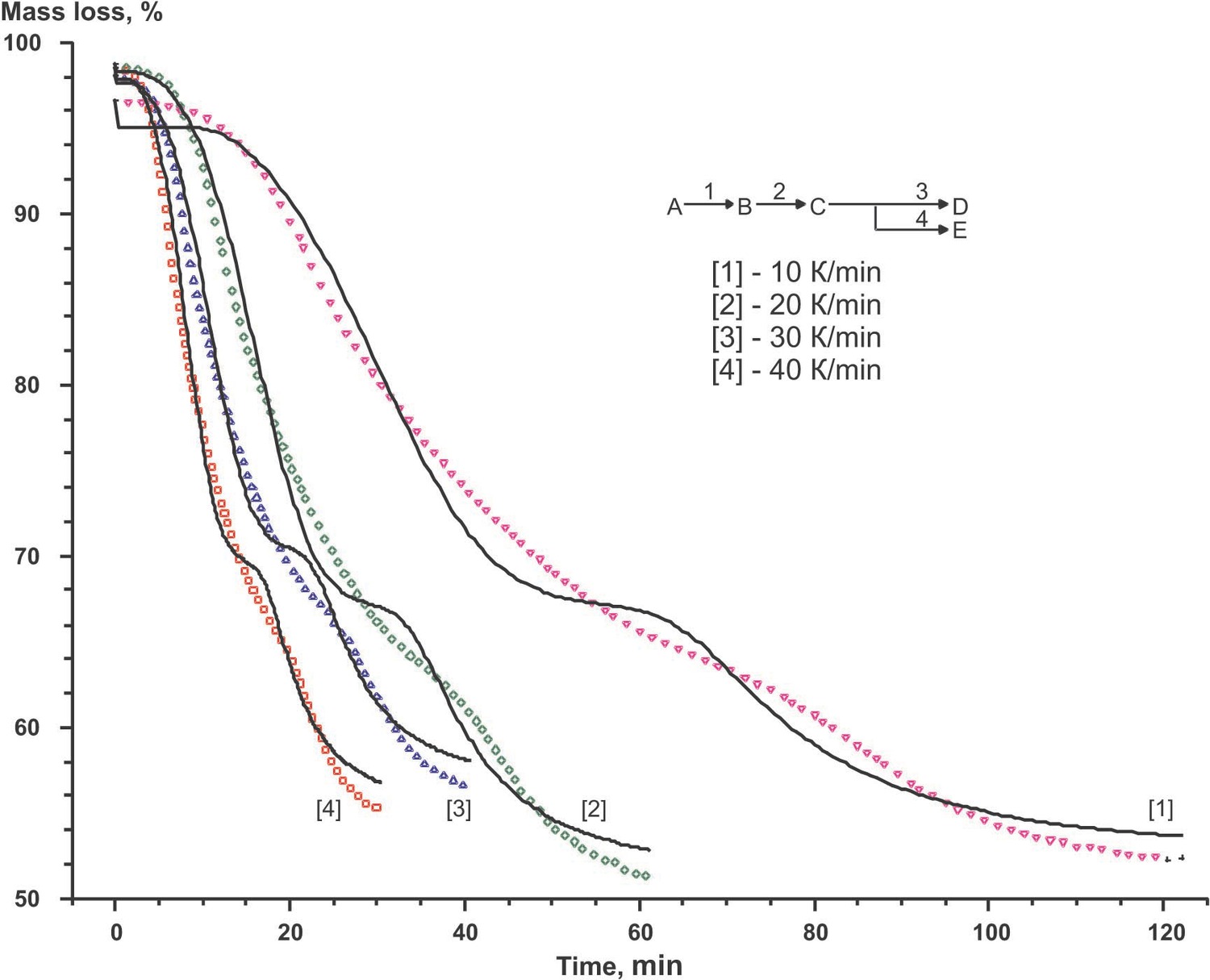
6.5 Calculated kinetic models and parameters of separate stages of the carbonization process for the successive-parallel scheme.
According to the authors [14] carbonization process may be represented by a set of successive-parallel processes. Let us consider this situation (the qffc scheme in Figure 3 of the Appendix). The results shown in Figure 6.3 and summarized in Table 6.5 have been obtained with the use of the same set of functions.
The F test value for the latter scheme with respect to the former one is
Fexp = 58.6, Ftheor = 1.11.
Comparison of the calculation results for each scheme reliably shows that, from the formal kinetic viewpoint, the scheme of successive stages best describes thermoanalytical data as a whole.
Thus, formal kinetic analysis makes it possible to choose the type of function best fitting the experimental curves (TG, DTG, DSC), evaluate kinetic parameters, determine the number of stages and their sequence (successive, parallel, etc.). In addition, the statistically optimal kinetic parameters allow one to model temperature change conditions resulting in constant weight loss or enthalpy change rate and obtain dependences of these characteristics under isothermal conditions or in other temperature programs.
6.2.1 References
[1] J. Sestak. Thermophysical Properties of Solids. Prague: Academia, 1984
[2] S. Vyazovkin al.. ICTAC Kinetics Committee Recommendations for Performing Kinetic Computations on Thermal Analysis Data Thermochimica Acta 1: 520 (2011): 520.
[3] V.A. Sipachev, I.V. Arkhangel ' skii. Calculation Techniques Solving Non-Isothermal Kinetic Problems Journal of Thermal Analysis 38: 1283-1291 (1992): 1283-1291.
[4] B. Delmon. Introduction to Heterogeneous Kinetics. Paris: Technip, 1969
[5] P. Barret. Kinetics in Heterogeneous Chemical Systems., 1974
[6] H.L. Friedman. A Quick, Direct Method for the Determination of Activation Energy from Thermogravimetric Data J. Polym. Lett. 4(5): 323-328 (1966): 323-328.
[7] T. Ozawa. A New Method of Analyzing Thermogravimetric Data Bull. Chem. Soc. Jpn. 38: 1881-1886 (1965): 1881-1886.
[8] J.H. Flynn, L.A. Wall. A Quick, Direct Method for the Determination of Activation Energy from Thermogravimetric Data J. Polym. Sci. Polym. Lett. 4: 323-328 (1966): 323-328.
[9] NETZSCH-Thermokinetics 3.1 Software Help. NETZSCH-Thermokinetics 3.1 Software Help. .
[10] J. Opfermann. Kinetic Analysis Using Multivariate Non-Linear Regression Journal of Thermal Analysis & Calorimetry 60: 641-658 (2000): 641-658.
[11] S.Z.D. Cheng. Handbook of Thermal Analysis and Calorimetry. Applications to Polymers and Plastics., 2001
[12] L. Shechter, J. Wynstra, J. W.. Glycidyl Ether Reactions with Amines Ind. Eng. Chem. 48: 94-97 (1956): 94-97.
[13] NETZSCH-Peakseparation 3.0 Software Help.. NETZSCH-Peakseparation 3.0 Software Help.. .
[14] P. Morgan. Carbon Fibers and Their Composites. New York: TaylorFrancis, 2005
[15] V.Y. Varshavskii. Carbon Fibers. Moscow: Varshavskii, 2005