Chemistry LibreTexts

3.5: Developing the Procedure

  • Page ID
    127191
  • \( \newcommand{\vecs}[1]{\overset { \scriptstyle \rightharpoonup} {\mathbf{#1}} } \)

    \( \newcommand{\vecd}[1]{\overset{-\!-\!\rightharpoonup}{\vphantom{a}\smash {#1}}} \)

    \( \newcommand{\id}{\mathrm{id}}\) \( \newcommand{\Span}{\mathrm{span}}\)

    ( \newcommand{\kernel}{\mathrm{null}\,}\) \( \newcommand{\range}{\mathrm{range}\,}\)

    \( \newcommand{\RealPart}{\mathrm{Re}}\) \( \newcommand{\ImaginaryPart}{\mathrm{Im}}\)

    \( \newcommand{\Argument}{\mathrm{Arg}}\) \( \newcommand{\norm}[1]{\| #1 \|}\)

    \( \newcommand{\inner}[2]{\langle #1, #2 \rangle}\)

    \( \newcommand{\Span}{\mathrm{span}}\)

    \( \newcommand{\id}{\mathrm{id}}\)

    \( \newcommand{\Span}{\mathrm{span}}\)

    \( \newcommand{\kernel}{\mathrm{null}\,}\)

    \( \newcommand{\range}{\mathrm{range}\,}\)

    \( \newcommand{\RealPart}{\mathrm{Re}}\)

    \( \newcommand{\ImaginaryPart}{\mathrm{Im}}\)

    \( \newcommand{\Argument}{\mathrm{Arg}}\)

    \( \newcommand{\norm}[1]{\| #1 \|}\)

    \( \newcommand{\inner}[2]{\langle #1, #2 \rangle}\)

    \( \newcommand{\Span}{\mathrm{span}}\) \( \newcommand{\AA}{\unicode[.8,0]{x212B}}\)

    \( \newcommand{\vectorA}[1]{\vec{#1}}      % arrow\)

    \( \newcommand{\vectorAt}[1]{\vec{\text{#1}}}      % arrow\)

    \( \newcommand{\vectorB}[1]{\overset { \scriptstyle \rightharpoonup} {\mathbf{#1}} } \)

    \( \newcommand{\vectorC}[1]{\textbf{#1}} \)

    \( \newcommand{\vectorD}[1]{\overrightarrow{#1}} \)

    \( \newcommand{\vectorDt}[1]{\overrightarrow{\text{#1}}} \)

    \( \newcommand{\vectE}[1]{\overset{-\!-\!\rightharpoonup}{\vphantom{a}\smash{\mathbf {#1}}}} \)

    \( \newcommand{\vecs}[1]{\overset { \scriptstyle \rightharpoonup} {\mathbf{#1}} } \)

    \( \newcommand{\vecd}[1]{\overset{-\!-\!\rightharpoonup}{\vphantom{a}\smash {#1}}} \)

    \(\newcommand{\avec}{\mathbf a}\) \(\newcommand{\bvec}{\mathbf b}\) \(\newcommand{\cvec}{\mathbf c}\) \(\newcommand{\dvec}{\mathbf d}\) \(\newcommand{\dtil}{\widetilde{\mathbf d}}\) \(\newcommand{\evec}{\mathbf e}\) \(\newcommand{\fvec}{\mathbf f}\) \(\newcommand{\nvec}{\mathbf n}\) \(\newcommand{\pvec}{\mathbf p}\) \(\newcommand{\qvec}{\mathbf q}\) \(\newcommand{\svec}{\mathbf s}\) \(\newcommand{\tvec}{\mathbf t}\) \(\newcommand{\uvec}{\mathbf u}\) \(\newcommand{\vvec}{\mathbf v}\) \(\newcommand{\wvec}{\mathbf w}\) \(\newcommand{\xvec}{\mathbf x}\) \(\newcommand{\yvec}{\mathbf y}\) \(\newcommand{\zvec}{\mathbf z}\) \(\newcommand{\rvec}{\mathbf r}\) \(\newcommand{\mvec}{\mathbf m}\) \(\newcommand{\zerovec}{\mathbf 0}\) \(\newcommand{\onevec}{\mathbf 1}\) \(\newcommand{\real}{\mathbb R}\) \(\newcommand{\twovec}[2]{\left[\begin{array}{r}#1 \\ #2 \end{array}\right]}\) \(\newcommand{\ctwovec}[2]{\left[\begin{array}{c}#1 \\ #2 \end{array}\right]}\) \(\newcommand{\threevec}[3]{\left[\begin{array}{r}#1 \\ #2 \\ #3 \end{array}\right]}\) \(\newcommand{\cthreevec}[3]{\left[\begin{array}{c}#1 \\ #2 \\ #3 \end{array}\right]}\) \(\newcommand{\fourvec}[4]{\left[\begin{array}{r}#1 \\ #2 \\ #3 \\ #4 \end{array}\right]}\) \(\newcommand{\cfourvec}[4]{\left[\begin{array}{c}#1 \\ #2 \\ #3 \\ #4 \end{array}\right]}\) \(\newcommand{\fivevec}[5]{\left[\begin{array}{r}#1 \\ #2 \\ #3 \\ #4 \\ #5 \\ \end{array}\right]}\) \(\newcommand{\cfivevec}[5]{\left[\begin{array}{c}#1 \\ #2 \\ #3 \\ #4 \\ #5 \\ \end{array}\right]}\) \(\newcommand{\mattwo}[4]{\left[\begin{array}{rr}#1 \amp #2 \\ #3 \amp #4 \\ \end{array}\right]}\) \(\newcommand{\laspan}[1]{\text{Span}\{#1\}}\) \(\newcommand{\bcal}{\cal B}\) \(\newcommand{\ccal}{\cal C}\) \(\newcommand{\scal}{\cal S}\) \(\newcommand{\wcal}{\cal W}\) \(\newcommand{\ecal}{\cal E}\) \(\newcommand{\coords}[2]{\left\{#1\right\}_{#2}}\) \(\newcommand{\gray}[1]{\color{gray}{#1}}\) \(\newcommand{\lgray}[1]{\color{lightgray}{#1}}\) \(\newcommand{\rank}{\operatorname{rank}}\) \(\newcommand{\row}{\text{Row}}\) \(\newcommand{\col}{\text{Col}}\) \(\renewcommand{\row}{\text{Row}}\) \(\newcommand{\nul}{\text{Nul}}\) \(\newcommand{\var}{\text{Var}}\) \(\newcommand{\corr}{\text{corr}}\) \(\newcommand{\len}[1]{\left|#1\right|}\) \(\newcommand{\bbar}{\overline{\bvec}}\) \(\newcommand{\bhat}{\widehat{\bvec}}\) \(\newcommand{\bperp}{\bvec^\perp}\) \(\newcommand{\xhat}{\widehat{\xvec}}\) \(\newcommand{\vhat}{\widehat{\vvec}}\) \(\newcommand{\uhat}{\widehat{\uvec}}\) \(\newcommand{\what}{\widehat{\wvec}}\) \(\newcommand{\Sighat}{\widehat{\Sigma}}\) \(\newcommand{\lt}{<}\) \(\newcommand{\gt}{>}\) \(\newcommand{\amp}{&}\) \(\definecolor{fillinmathshade}{gray}{0.9}\)

    After selecting a method, the next step is to develop a procedure that accomplish our goals for the analysis. In developing a procedure we give attention to compensating for interferences, to selecting and calibrating equipment, to acquiring a representative sample, and to validating the method.

    Compensating for Interferences

    A method’s accuracy depends on its selectivity for the analyte. Even the best method, however, may not be free from interferents that contribute to the measured signal. Potential interferents may be present in the sample itself or in the reagents used during the analysis.

    When the sample is free of interferents, the total signal, Stotal, is a sum of the signal due to the analyte, SA, and the signal due to interferents in the reagents, Sreag,

    \[S_{total} = S_A + S_{reag} = k_A n_A + S_{reag} \label{3.1}\]

    \[S_{total} = S_A + S_{reag} = k_A C_A + S_{reag} \label{3.2}\]

    Without an independent determination of Sreag we cannot solve Equation \ref{3.1} or \ref{3.2} for the moles or concentration of analyte.

    To determine the contribution of Sreag in Equations \ref{3.1} and \ref{3.2} we measure the signal for a method blank, a solution that does not contain the sample. Consider, for example, a procedure in which we dissolve a 0.1-g sample in a portion of solvent, add several reagents, and dilute to 100 mL with additional solvent. To prepare the method blank we omit the sample and dilute the reagents to 100 mL using the solvent. Because the analyte is absent, Stotal for the method blank is equal to Sreag. Knowing the value for Sreag makes it is easy to correct Stotal for the reagent’s contribution to the total signal; thus

    \[(S_{total} - S_{reag}) = S_A = k_A n_A \nonumber\]

    \[(S_{total} - S_{reag}) = S_A = k_A C_A \nonumber\]

    By itself, a method blank cannot compensate for an interferent that is part of the sample’s matrix. If we happen to know the interferent’s identity and concentration, then we can be add it to the method blank; however, this is not a common circumstance and we must, instead, find a method for separating the analyte and interferent before continuing the analysis.

    A method blank also is known as a reagent blank. When the sample is a liquid, or is in solution, we use an equivalent volume of an inert solvent as a substitute for the sample.

    Calibration

    A simple definition of a quantitative analytical method is that it is a mechanism for converting a measurement, the signal, into the amount of analyte in a sample. Assuming we can correct for interferents, a quantitative analysis is nothing more than solving Equation 3.3.1 or Equation 3.3.2 for nA or for CA.

    To solve these equations we need the value of kA. For a total analysis method usually we know the value of kA because it is defined by the stoichiometry of the chemical reactions responsible for the signal. For a concentration method, however, the value of kA usually is a complex function of experimental conditions. A calibration is the process of experimentally determining the value of kA by measuring the signal for one or more standard samples, each of which contains a known concentration of analyte.

    With a single standard we can calculate the value of kA using Equation 3.3.1 or Equation 3.3.2. When using several standards with different concentrations of analyte, the result is best viewed visually by plotting SA versus the concentration of analyte in the standards. Such a plot is known as a calibration curve, an example of which is shown in Figure 3.5.1 .
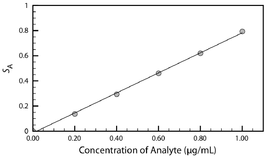
    Figure 3.5.1 : Example of a calibration curve. The filled circles (•) are the results for five standard samples, each with a different concentration of analyte, and the line is the best fit to the data determined by a linear regression analysis. See Chapter 5 for a further discussion of calibration curves and an explanation of linear regression.

    Sampling

    Selecting an appropriate method and executing it properly helps us ensure that our analysis is accurate. If we analyze the wrong sample, however, then the accuracy of our work is of little consequence.

    A proper sampling strategy ensures that our samples are representative of the material from which they are taken. Biased or nonrepresentative sampling, and contaminating samples during or after their collection are two examples of sampling errors that can lead to a significant error in accuracy. It is important to realize that sampling errors are independent of errors in the analytical method. As a result, we cannot correct a sampling error in the laboratory by, for example, evaluating a reagent blank.

    Chapter 7 provides a more detailed discussion of sampling, including strategies for obtaining representative samples.

    Validation

    If we are to have confidence in our procedure we must demonstrate that it can provide acceptable results, a process we call validation. Perhaps the most important part of validating a procedure is establishing that its precision and accuracy are appropriate for the problem we are trying to solve. We also ensure that the written procedure has sufficient detail so that different analysts or laboratories will obtain comparable results. Ideally, validation uses a standard sample whose composition closely matches the samples we will analyze. In the absence of appropriate standards, we can evaluate accuracy by comparing results to those obtained using a method of known accuracy.

    You will find more details about validating analytical methods in Chapter 14.


    This page titled 3.5: Developing the Procedure is shared under a CC BY-NC-SA 4.0 license and was authored, remixed, and/or curated by David Harvey.

    • Was this article helpful?