22.1: Carbon-13 NMR

The following table shows the spin quantum numbers of several nuclei. Only elements that have a nuclear spin quantum number I other than zero are NMR active. Such elements have odd atomic number, or odd atomic mass, or both. Elements whose atomic number and atomic mass are both even have I = 0 and are not NMR active.

 

SPIN QUANTUM NUMBERS OF COMMON NUCLEI

	^11H	^21H	^126C	^136C	^147N	^168O	^178O	^199F	^3115P	^3517Cl
Nuclear spin quantum (I)	1/2	1	0	1/2	1	0	5/2	1/2	1/2	3/2
Number of spin states n=2I  + 1	2	3	0	2	3	0	6	2	2	4

Because both proton and carbon have the same nuclear spin value, they behave similarly in NMR and similar guidelines apply to the analysis of their spectra. However, there are also some important differences. Examination of the following table reveals the basis for some of those differences.

 

FIELD STRENGTHS AND RESONANCE FREQUENCIES FOR SELECTED NUCLEI

Isotope	Natural Abundance (%)	Field Stength (Bo) in Tesla*	Absorption Frequency (v) in MHz
^1H	99.98	1.00 2.35 4.70 7.05	42.6 100 200 300
^2H	0.02	1.00	6.5
^13C	1.11	1.00 2.35 4.70 7.05	10.7 25 50 75
^19F	100	1.00	40
^31P	100	1.00	17

*1 Tesla = 10,000 Gauss

Natural abundance effect. The natural abundance of proton means that virtually all the hydrogen atoms in a molecule are the 1 H isotope, and therefore are in high abundance. This in turn means that a good NMR signal can be obtained in relatively short times with samples of relatively low concentrations. Conversely, the low natural abundance of the ¹³C isotope means that most of the carbon atoms in a molecule are of the ¹²C kind, which is NMR inactive. In order to obtain a good ¹³C NMR signal longer times and more concentrated samples are required.

Absorption frequency effect. The table also shows that the absorption frequency for carbon is about 1/4 that of proton for a given magnetic field strength. The absorption frequency represents a very narrow window where all the atoms of the same kind in a molecule can be observed. This in turn means that when observing ¹H, carbon will be invisible, and vice versa.

Chemical shift range. Another difference between proton and carbon is in the effect of the functional groups and the electronegativity of other atoms on these nuclei. Let’s say that there is a carbonyl group (C=O) present in a molecule. The deshielding effect of the oxygen atom, for instance, is most strongly felt by carbon, since it’s directly attached to the oxygen atom. Any hydrogen atoms present in the neighborhood of the carbonyl group will experience a lessened effect from the oxygen due to increased distance from it. In general, because carbon comprises the molecular skeleton to which other atoms and functional groups are attached, it will experience the shielding or deshielding effects of these groups more intensely than proton. This in turn means that the chemical shift range for carbon is more spread out than for proton. Most of the proton types observed in common organic molecules lie within a range of 0-15 ppm in the chemical shift (δ scale). Carbon atoms, conversely, lie within a range of 0-200 ppm. Refer to fig. CMR.2 on page A52 of your laboratory textbook.

Signal intensity considerations. Unlike proton NMR, the signal intensities for carbon are not necessarily representative of the relative proportions of different types of carbons in the molecule. This effect stems from the relaxation time –the time that it takes for a nucleus in the β state to revert back to the α state after the application of a radiofrequency pulse. The relaxation times for carbon are much longer than for proton. Because of practical considerations, this means that the signal intensities in a typical carbon spectrum do not represent the relative proportions of the different types of carbon, unless special conditions are carefully implemented.

Signal multiplicity. The multiplicity of signals observed in proton NMR is primarily due to proton-proton coupling. Due to the high natural abundance of protons, the probability that two ¹H nuclei be neighbors is practically 100%. They will split each other’s signals if they are coupled and if they are chemically non equivalent. The situation for carbon is different. The extremely low natural abundance of carbon-13 means that the probability that two ¹³C nuclei be next to each other in the molecule is practically nonexistent. Thus ¹³C nuclei do not split each other. However, if there are ¹H nuclei directly attached to ¹³C they will cause signal splitting. This carbon-proton splitting follows the same rules as proton-proton splitting, since both nuclei have the same nuclear spin quantum number. This means that in general, a carbon atom that has no hydrogen atoms directly attached to it will be a singlet. A carbon atom that has one hydrogen atom attached to it will be a doublet, and so on (n + 1 rule applies).

Furthermore, carbon spectra can be run in one of two modes, proton-coupled and proton-decoupled. In the proton-coupled mode carbon signals experience splitting. In the proton-decoupled mode they do not and they appear as singlets, regardless of how many hydrogen atoms are attached to a given carbon. One problem that arises with proton-coupled carbon signals is that their coupling constants are much larger than those of proton, causing overlap with other signals and confusion as to which peaks being observed are for the same signal and which are for different signals. To solve this problem, a technique referred to as “off-resonance decoupling” is used. The coupling constants obtained in this way are much smaller than normal and the problem of overlapping signals becomes much less severe.

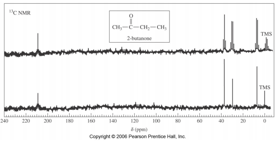
The spectrum on the following page illustrates this concept. The bottom portion represents the proton-decoupled spectrum of 2-butanone, showing only four singlets, corresponding to four different types of carbons in the molecule. The spectrum at the top is the “off-resonance decoupled” spectrum, showing the same signals, but also their multiplicities, reflecting to the number of hydrogens attached to each carbon (two quartets for the two methyl groups, one triplet for the –CH₂ – group, and one singlet for the C=O group).

For another example refer also to fig. CMR.1 on p. A51 of your laboratory textbook.

The proton-decoupled carbon NMR spectra for camphor, borneol, and isoborneol are shown in your lab textbook on pages 275 and 276.​​​​​​​