
2.2 Experiment 1 and 2 Procedures
- Page ID
- 212013
\( \newcommand{\vecs}[1]{\overset { \scriptstyle \rightharpoonup} {\mathbf{#1}} } \) \( \newcommand{\vecd}[1]{\overset{-\!-\!\rightharpoonup}{\vphantom{a}\smash {#1}}} \)\(\newcommand{\id}{\mathrm{id}}\) \( \newcommand{\Span}{\mathrm{span}}\) \( \newcommand{\kernel}{\mathrm{null}\,}\) \( \newcommand{\range}{\mathrm{range}\,}\) \( \newcommand{\RealPart}{\mathrm{Re}}\) \( \newcommand{\ImaginaryPart}{\mathrm{Im}}\) \( \newcommand{\Argument}{\mathrm{Arg}}\) \( \newcommand{\norm}[1]{\| #1 \|}\) \( \newcommand{\inner}[2]{\langle #1, #2 \rangle}\) \( \newcommand{\Span}{\mathrm{span}}\) \(\newcommand{\id}{\mathrm{id}}\) \( \newcommand{\Span}{\mathrm{span}}\) \( \newcommand{\kernel}{\mathrm{null}\,}\) \( \newcommand{\range}{\mathrm{range}\,}\) \( \newcommand{\RealPart}{\mathrm{Re}}\) \( \newcommand{\ImaginaryPart}{\mathrm{Im}}\) \( \newcommand{\Argument}{\mathrm{Arg}}\) \( \newcommand{\norm}[1]{\| #1 \|}\) \( \newcommand{\inner}[2]{\langle #1, #2 \rangle}\) \( \newcommand{\Span}{\mathrm{span}}\)\(\newcommand{\AA}{\unicode[.8,0]{x212B}}\)
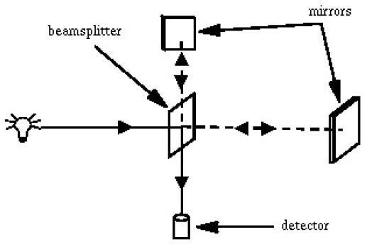
Experiment 1. What's in the Spectrometer?
Identify elements of the spectrometer shown in the figure below in the open spectrometer unit and identify the path of the light.
Experiment 2. Lambert-Beer's Law
- Prepare 0.01, 0.02, 0.03, 0.04 and 0.05 M aqueous solutions of \(CoCl_2\) in volumetric flasks. When making up your solutions, note that you will be using cobalt chloride hexahydride (\(CoCl_2 \cdot 6H_2O\)) and be sure to use the proper molecular mass in your calculations. Your TA will prepare a solution with unknown concentration, between 0.01 and 0.05 M.
- Make sure that the absorbance spectrometer is plugged in and connected to the computer via USB port - you should be able to hear its fan running - and open the SpectraSuite program. Fill a cuvette with water, wipe the sides of the cuvette with a Kimwipe, and place the cuvette in the holder.
- Under the Spectrometer menu select Rescan Devices. Find the absorbance spectrometer picture, expand menu [+], and expand Properties [+] to check that the serial number corresponds to the spectrometer. Right click on any other spectrometers and select Remove Spectrometer. Right click on any other spectrometer and select Remove Spectrometer. If there is no graph on the screen, right click the spectrometer picture and choose Show Graph.
- Click the Pause [
 ] button and change the parameters at the top of the screen to Integration Time = 10 ms, Average = 10, and Boxcar = 10. Check the Electric Dark Correction box. This box should remain checked throughout all experiments.
 - Click Play [
 ] to begin the acquisition. When you no longer see major fluctuations in the spectrum over time, click on the dark light bulb [
 ] to store the dark reference spectrum. Check Strobe/Lamp Enable Box and repeat, clicking on the yellow light bulb [
 ] to store reference spectrum. Now the Absorbance [
 ] icon should be accessible. Click it to enter absorbance mode and then click Pause.
 - Remove and empty your cuvette. Wash with your first sample solution, empty, and then fill with the solution. Place in holder.
- Take a spectrum by clicking Play, then clicking Pause when your feel you have a good spectrum. You can change the viewing parameters of the graph using [
 ] to auto-scale, [
 ] to vertically scale the spectrum, [
 ] to manually set the zoom parameters, and [
 ] to toggle and pan the spectrum. You can also zoom in and out of the graph using the scrolling wheel on the mouse.
 - Click the Save [
 ] icon to save this spectrum. Don't access this function through the File menu. Under Desired Spectrum, select Processed Spectrum and make sure that file type is ''.OOI" and the appendage to the file name is ".ProcSpec" before pressing Save. If the Save button isn't activated, try clicking elsewhere in the Save window first.
 - Remove, empty, and rinse the cuvette with your next sample. Fill the cuvette with the new solution, acquire a new spectrum, and save. Continue for all samples of solution.
- After all spectra have been taken, click Overlay Spectral Data [
 ] icon and select one of your saved spectra. Select Processed and then click
  . Repeat for all of your processed spectra. This should overlay all of your spectra onto the same graph.
 - Click on the spectrum graph area, then type "510" into the Wavelength (nm) text window at the bottom of the screen and hit enter. The absorbance values of your overlaid spectra at 510 nm will appear to the right of the text window in their respective colors. Record these values in your notebook.
- Do a linear fit to the function \(A = f(c)\). Read off the value of the absorbance for the unknown sample and using the fit calculate its concentration. What is the approximate uncertainty of the measurement? What do you think the biggest sources of error are?