1.2 - Background

Light and Matter

What happens when a sample is irradiated by light? From introductory chemistry courses, you might have a quantum mechanical picture of light absorption, which emphasizes that light energy comes in quantized units, called photons, and that a molecule’s energy also comes in quantized units or “quanta”, so when a molecule absorbs a photon, it takes up the photon’s energy to reach an “excited state” of some sort. Your picture of light absorption might look like this.

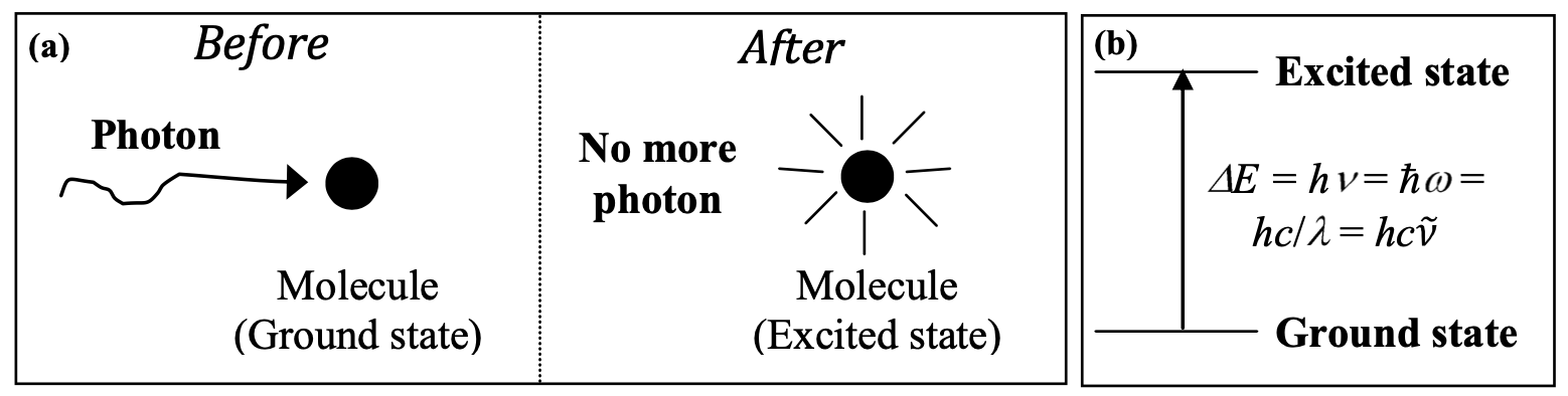Figure 1: Optical Absorption

Both of these depictions get one crucial element correct: conservation of energy. The photon energy does indeed get turned into molecular energy. Also, since molecular energy is quantized, there are only molecular excited states at certain discrete energy levels. The photon energy has to be equal to the difference \(\Delta E\) between some pair of energy levels of the molecule in order for absorption to occur. There are many types of states that these energy levels could correspond to, but in this module, you will only consider electronic, vibrational, and spin states.

Exercise 1

What are the names, values, and units of \(h\) and \(\hbar\)? How about \(\nu\), \(\omega\), \(\lambda\) and \(\tilde{\nu}\)? What are their values for visible and infrared light and for the MIT radio station frequency?

Figure 1 also contains some grave simplifications. Its biggest problem is that it suggests that the molecule is in a static, or (in quantum mechanical terms) stationary, excited state after irradiation. The accuracy of this description varies, but in your NMR experiments, you will see graphic evidence that it is not complete. In those experiments, you will irradiate a sample with a pulse of radiation at radio frequencies (RF) and you will measure the time-dependent, oscillating state of the proton spins in the sample, long after the RF pulse is gone. Similarly, time-dependent molecular vibrations that occur during and after irradiation by an IR pulse can be measured, although their time scale is so fast that ultrashort laser pulses are required to observe the individual vibrational oscillations. Time-dependent oscillations in molecular electronic charge distribution due to visible or UV light are even faster, but there are ways of measuring them too.

Exercise 2

Express the frequency values ν that you found from Exercise 1 in reasonable units, i.e. megahertz (\(MHz\)), gigahertz (\(GHz\)), or terahertz (\(THz\)). Now calculate the time \(T\) required for a single oscillation period in each case, again expressed in appropriate units of microseconds (\(\mu s\)), nanoseconds (\(ns\)), picoseconds (\(ps\)), or femtoseconds (\(fs\)). These are the frequencies and oscillation periods of the RF, IR, and visible radiation and also of the respective spin, vibrational, and electronic responses of molecules that have energy levels whose differences match the radiation frequencies. When molecules are irradiated at a frequency that matches a transition between two energy levels, we say that the radiation is on resonance with the molecular transition frequency.

Exercise 3

Indicate what types of molecular energy level transitions are involved in the following spectroscopic techniques: NMR, IR, UV-Vis, Fluorescence.

These dynamical, time-dependent responses can be expressed in the most accurate and general terms through time-dependent quantum mechanics, which isn’t treated in undergraduate courses. Fortunately, it can be expressed with excellent accuracy in most cases in the framework of classical mechanics. And this is something for which you have a lifetime of experience and intuitive understanding.

Figure 2 is an alternate depiction of light absorption. This picture is very different from those in Figure 1! Light is now depicted as a propagating wave, not a particle. The molecule is now shown as a classical harmonic oscillator, suggesting any possible vibrational amplitude, rather than only a set of discrete states. Which picture is right?

Figure 2: Optical Adsorption

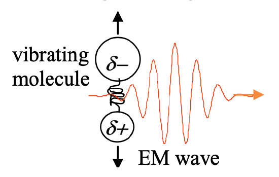
The answer is that both pictures are correct, and both can offer important insights. Figure 2 correctly suggests that light is a propagating electromagnetic wave. The molecule does indeed respond to the light much as a harmonic oscillator would. For example, a polar molecule like HCl responds to an oscillating electric field by alternately stretching and compressing, that is, through well-defined vibrational oscillations induced at the frequency of the field. The induced oscillation amplitude is proportional to the amplitude of the light field. If the light frequency is on or near the molecular vibrational resonance frequency, the induced oscillations are larger in amplitude than if the light frequency is far off resonance. Experiments can be conducted that permit direct observations of these time-dependent vibrational oscillations.

If we can view the irradiated molecule as a classical oscillator responding to a classical force exerted by a classical electromagnetic field, what about the quantum mechanical view? The details of this discussion will have to wait until 5.61 and even beyond, but the basic results can be described here. The molecule does indeed have well defined stationary states with well defined, discrete energies, as depicted in Fig. 1b. Molecular and light energy do come in discrete quanta as that figure suggests. But the fact that the molecule has time-independent, stationary states does not mean that the molecule always must be in one of those states. The molecule may be in a time-dependent state, which is not one of the stationary states but is described mathematically as a linear combination of stationary states. The time-dependent state may be very much like a classical oscillator, and any oscillation amplitude is possible. This may seem to suggest that any vibrational energy is possible, in contrast to the laws of quantum mechanics. But it turns out that if you make a measurement of molecular vibrational energy, you always get one of the discrete energy values corresponding to one of the stationary states. Similarly, it is accurate to describe the light coming from a lamp or a laser as an oscillating electromagnetic field that can drive oscillating molecular responses. But if you measure the energy taken up by a molecule when it absorbs light, you find that the energy comes in indivisible quanta – what we call photons.

The reconciliation of time-dependent, classical molecular vibration and classical electromagnetic waves with quantized molecular energy levels and photons is a subtle point, but rest assured that the two apparently contrasting views presented in Figures 1 and 2 are indeed compatible. And that means we should not disregard Figure 2, for which life in the classical world has provided us ample intuition. Infrared light really does drive molecular vibrational oscillations. Visible and UV light drive electron clouds to move in an oscillatory fashion about their host nuclei. RF radiation drives magnetic dipoles in an oscillatory fashion, as any oscillating magnetic field drives a bar magnet. Where possible, we will use classical mechanics to explain spectroscopy.

 

Electromagnetic Radiation and the Electromagnetic Spectrum

Since light can be described as an electromagnetic wave, we should be able to depict it and understand parameters like those of Figure 1, applied to individual photons, in terms of wave motion. Imagine a wave propagating through space in what we will define as the x direction. We can describe the electric field as follows;

\[\mathbf{E}(x, t)=\widehat{\boldsymbol{\varepsilon}} E_{0} \cos (k x-\omega t)\]

Let’s look at this equation. First, the field is a vector (bold); it is directional. On the RH side, first, we see a unit vector that indicates the direction along which the field is pointed. Here we’ve written \(\widehat{\boldsymbol{\varepsilon}}\)as time-independent for simplicity. Next, we see an amplitude \(E_0\), which we also have chosen to make time-independent. This describes a never-ending wave of light with a time-independent amplitude; later we’ll describe pulses of light whose amplitudes are time-dependent. Finally, we have the oscillatory cosine term that indicates that the field is an oscillating function of both position and time. If we pick any position in space (fix the value of \(x\)) we see that the field that passes through that point oscillates in time. If we pick a fixed time, we see that the field oscillates in position.

Exercise 4

Plot the field as a function of time at a fixed position and vice versa. Indicate the amplitude \(E_0\) and the oscillation period \(T\) for the first plot and the wavelength \(\lambda\) for the second. What are the relationships between \(T\) and \(\omega\) and \(\nu\) and between \(\lambda\) and \(k\), the wavevector?

Absorption of Light

How do we describe how light interacts with molecules? Sticking with our classical picture, let’s start with F = ma. In this case, the force exerted is the time-dependent, oscillating electromagnetic field. Let’s consider the molecular vibrations of a polar, diatomic molecule like HCl. Treating it as a harmonic oscillator, we can write its equation of motion including three force terms: the Hooke’s Law restoring force due to the spring, a frictional damping term proportional to the velocity, and the external force applied by the light. The result is

\[\mu \frac{d^{2} Q}{d t^{2}}+b \frac{d Q}{d t}+K Q=a E_{0} \cos (\omega t)\]

 where Q, the vibrational coordinate, is the deviation from the equilibrium length of the spring (or the equilibrium bond length), μ is the reduced mass of the molecule, b is a friction coefficient, K is the force constant, and a is a coupling constant that measures how effectively the light drives the molecular vibration. We don’t need to include propagation of the light or the position of the molecule explicitly in this equation; we can just solve it for any position (i.e., x = 0), and assume it will be the same everywhere else. Also note that the bigger a is, the larger the amplitude of vibration. We won’t go into detail about this coupling constant here, except to mention that it depends on how polar the vibration is. The dipole moment of the molecule has to change as a result of the vibrational motion for the mode to be IR-active, that is, for it to absorb any IR light at all. Therefore, vibrations in homonuclear diatomics like H2 and Br2 do not appear in IR spectra (in our equation of motion, a = 0). The molecules vibrate but there is no change in dipole moment when they do. The result is that an electric field does not exert a force that affects the bond.

Extra Exercise 1

This is your chance to “do the math.” It is the fundamental classical mechanics of a driven, damped oscillator, which is an important problem that comes up in myriad contexts. It is somewhat time-consuming but straightforward since you are expected to use a text or online treatment from which you can follow the derivations and transcribe them directly. However, it is expected that you understand clearly anything you turn in.

Find a treatment of the classical mechanics of a driven, damped harmonic oscillator.

1. Show for a mass m that is connected by a spring of force constant K to an infinitely massive, immovable wall, that Newton’s Law F = ma along with Hooke’s Law F = - KQ (where Q measures the stretching of the spring, starting from its length with the mass at rest) yield the equation of motion \(m \frac{d^{2} Q}{d t^{2}}+b \frac{d Q}{d t}+K Q=0\) where the second term, which you will see describes damping, has simply been added in. Then show that for two masses, m1 and m2, on the two ends of the spring, the equation of motion has the same form \(\mu \frac{d^{2} Q}{d t^{2}}+b \frac{d Q}{d t}+K Q=0\), where the mass m has been replaced by the reduced mass μ for which you should derive an expression.

2. Show that with no friction, i.e. b = 0, the solutions are oscillatory at the resonance frequency \(\omega_{0}=\sqrt{\frac{K}{\mu}}\). If you stretch the oscillator by some amount Q0 and then let go (i.e. set initial conditions \(Q=Q_{0}, d Q / d t=0\), the solution takes the form \(Q(t)=Q_{0} \cos \left(\omega_{0} t\right)\). 

3. Show that for weak friction, the solutions are exponentially damped oscillations: \(Q(t)=Q_{0} e^{-\gamma t} \cos (\Omega t)\), where \(\gamma=\frac{b}{2}\) is the damping constant and the oscillation frequency  \(\Omega = \sqrt{\omega_0^2 - \gamma^2}\) is slightly lower than the resonance frequency. 

How does the harmonic oscillator respond to a periodic driving force like that exerted by light? It is possible to use eq. (2) to derive the response of the damped harmonic oscillator to an oscillating driving force at the driving frequency \(\omega\). The result is

\[ Q(t)=A(\omega) \sin (\omega t+\beta)\]

with the vibrational amplitude, \(A\) increasing as the driving frequency approaches the resonance frequency \(\omega_0\). The vibrational amplitude depends on the driving field amplitude and on the driving frequency,

\[A(\omega)=\frac{a E_{0} / \mu}{\left(\left(\omega^{2}-\omega_{0}^{2}\right)^{2}+4 \gamma^{2} \omega^{2}\right)^{1 / 2}}\]

Finally, the amount of power that is absorbed from the driving field by the damped oscillator is given in classical mechanics by the expression \(power = force * velocity\). Using our expressions above and neglecting oscillations that are very rapid in comparison to the length of the measurement (that is, averaging over an oscillation period), we get

\[P(\omega)=\frac{\left(a E_{0}\right)^{2}}{\mu} \frac{\gamma \omega^{2}}{\left(\omega^{2}-\omega_{0}^{2}\right)^{2}+4 \gamma^{2} \omega^{2}} \approx \frac{\left(a E_{0}\right)^{2}}{4 \mu} \frac{\omega^{2}}{\left(\omega-\omega_{0}\right)^{2}+\gamma^{2}}\]

assuming weak damping and a driving frequency that is near resonance. Maximum power absorption occurs on resonance, and the power absorbed far from resonance is negligible. In an absorption spectrum, you measure how much power \(P(\omega)\) from a light source is absorbed by the sample as a function of the light frequency. The functional form on the RH side of eq. (5) is called a Lorentzian function. Its peak is at the resonance frequency \(\omega_0\) and its width is given by the damping constant \(\gamma\). Thus the basic parameters of the sample can be determined directly from the absorption spectrum. Note that the power absorbed depends on the field amplitude squared, or the light intensity, which, averaged over the cycles of the field, is the light power. That is, the amount of power absorbed is proportional to the amount of power that hits the sample.

Extra Exercise 2

Plot the time-dependent displacement of the damped harmonic oscillator \(Q(t)\). Plot the frequency-dependent vibrational amplitude and power absorption for the driven oscillator with \(\gamma = \omega_0/10\) and \(\omega_0/100\). Indicate the parameters \(\omega_0\) and \(\gamma\) on the frequency plots. What changes in these plots as \(\omega\) change?

Note that in the treatment above, we wrote that the driving force oscillates as \(cos(\omega t)\)while the driven response oscillates as \(sin(\omega t + \beta)\). The frequencies are the same, but the vibrational phase may not be. When the vibrational phase factor \(\beta\) is \(\pm \pi/2\), \(sin(\omega t + \beta) = cos(\omega t)\)and the driving force and the response are in phase. This happens whenever the driving frequency is far off-resonance. On the other hand, when \(\beta = 0 \), the response is 90\(^o\) out of phase with the driving force and the driving frequency is exactly on resonance. This is one way of thinking about the power absorbed from the driving force: it is largest when the frequency is on resonance because the force is always driving the oscillator out of phase, and therefore always meeting substantial resistance.

In the classical damped harmonic oscillator, the time-dependent oscillations and the vibrational energy are damped at a rate given by \(\gamma\). When damping is complete, there are no significant further oscillations and the vibrational energy is zero. We say that the well- defined time-dependent oscillations treated above are phase-coherent because their timing—their vibrational phase, \(\beta\)—is well defined. It turns out that the absorption line width \(\gamma\) really measures the loss of vibrational phase-coherence, or dephasing (sometimes called “decoherence”). In some cases the dephasing rate and the energy decay rate are the same, but in many cases dephasing is much faster. This is the case with electronic and spin states as well as vibrations. The absorption linewidths tell us about how long it takes for the coherent oscillations in vibrational displacement, electronic charge distribution, or magnetic moment to decay, but not about how long the vibrational, electronic, or spin energy is retained by the molecule (vibrational, electronic, or spin state lifetimes).

We should not forget entirely the quantum mechanical picture, e.g. Fig. 1b. The resonance frequency ω0 that we associate with classical time-dependent oscillations also gives us the energy difference, \(\Delta E = \hbar \omega_0\), between the ground state and an excited state of the molecule. The reason that energy might remain in the molecule long after coherent oscillations are fully damped is that the molecule at that point may be left in the excited state – a stationary state. The energy lifetime is just the lifetime of the molecule in that state. Eventually the molecule will return to the ground state by some mechanism – emission of light (fluorescence) or a nonradiative mechanism in which the energy is lost to the thermal energy of the surroundings.