Bits, Noise, and Linearity; the Imperfections of ADCs

Now that we've seen how a variety of ADCs work, how can we compare and contrast their behavior? Comparisons can be drawn in many ways:

Number of useful bits and encoding scheme

Just because an ADC is physically wired for some number of bits does not necessarily mean that all those bits will be valid under all circumstances. Suppose we think of a 16 bit successive approximations ADC. 3/4 of the way through doing a conversion, the 12 most significant bits have been set. If we simply read out those bits, we have used a 16 bit device to do a 12 bit conversion. Any successive approximations or Σ-Δ scheme be modified so that one can sacrifice resolution in order to gain speed (or vice versa). Similarly, a V to F converter may have hardware allowing, say, 20 bits resolution for a 1 V full scale measurement lasting 10 s. That same hardware would measure 17 bits in 1.25 s (1/8 time = (1/2)³, so 3 fewer bits).

Exercise: For the V to F system described above, how long would it take to do an 8 bit conversion?

Click for answer
and explanation

Given the answer to the first part of this exercise, if you only wanted 8 bits resolution, would you choose this V to F system or a flash converter?

Click for answer
and explanation

The coding scheme matters as well. A 12 bit converter, operating in 2's complement binary mode, generates 11 bits of magnitude information, plus a sign bit. But what if we know the sign of the data in advance? Then coding in straight binary gives the potential for twice the resolution in the measurement. If the ADC codes as offset binary but the computer to which it is interfaced uses 2's complement binary, software to convert each incoming piece of data is required, slowing down data reduction. If an ADC is to directly drive a digital display, one must know if the display controller expects straight binary (plus sign), offset binary, or 2's complement binary coding, or the display will be in error even if the ADC is working correctly. Finally, some displays expect decimal input. While we did not discuss ADCs that directly digitize in decimal, they do exist (wasting coding space -- the highest resolution for transistor or lead possible is with binary coding).

Digitization rate (frequency)

How rapidly does the ADC refresh its output? That's the digitization rate. Approximate rates are tabulated below (but one must look at the specifications for each system; just knowing the type isn't enough!).

ADC Type	Number of bits	Digitization Rate (Hz)
Dual Slope	12-18	1-100
V to F	12-24	1-1000
Successive Approximations	12	10^5 - 20×10^6
	16	10^4 - 4×10^6
Flash	8	10^6 - 10^8
Σ Δ	14-24	1-1.92×10^5

In general, higher resolution correlates with slower conversion. Some compound types (pipelined converters) may mix a flash converter for the most significant bits with some other strategy for less significant bits.

Bandwidth (not necessarily the same as digitization rate)

What is the Nyquist frequency for the ADC system? That depends on the analog circuitry preceding the converter. If the analog circuitry has an RC time constant longer than the time between conversions, then that circuitry sets the effective bandwidth of the ADC. Higher analog frequencies are suppressed, reducing the likelihood of aliasing. On the other hand, if the analog system is fast, the Nyquist frequency becomes 1/2 the sampling frequency. Thus, a successive approximations ADC sampling at 1 MHz has a Nyquist frequency of 500 kHz unless a slower analog front end reduces the frequency to below this value. As with many compound systems, if both front end and sampling are important, the overall Nyquist frequency is a root-mean-square combination of the components. One must be a bit careful; the SLOWEST component dominates. Thus Δν²_{Nyquist,total}=(Δν^-2_{Nyquist,Analog} + Δν^-2_{Nyquist,Digital})^-2. Note that if the analog Nyquist frequency is above the digital Nyquist frequency, aliasing will occur and data interpretation must include analysis of this effect.

Linearity, missed codes

It is natural to expect that even if an ADC is inaccuracte, at least its output will change smoothly from low to high as an input changes from low to high. For V to F converters, and for dual slope converters not near 0 volts, this expectation is met However, near zero cross-over, for some inputs on successive approximation converters, for some flash converters, and for some conditions on higher order Σ-Δ units, non-monotonic behavior can occur. An example is shown below, where the resistor for the 3rd-least significant bit of a successive approximations unit has an error, so that there is a jump in output for certain specific small changes in input.

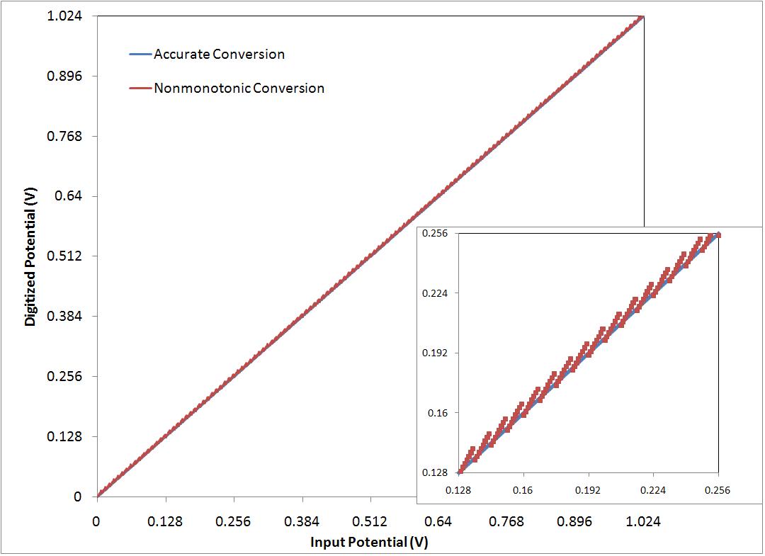
The linearity specification of an ADC is the root-mean-square difference between true linear response and the actual readout. One hopes the output is:

\[\mathrm{Count = Offset + k \times V_{in}}\]

If there is continuously varying nonlinearity over the range of the converter, a better model for the output is:

\[\mathrm{Count = Offset + k_L \times V_{in} + k_Q \times V^2_{in}}\]

For the situation we see in the graph above, the problem isn't large-scale nonlinearity, but rather discontinuities in the conversion. Here, simply looking at the short-range slope of conversion per change in potential input and comparing it to the overall average indicates that there's a patterned error.

Signal-to-noise ratio

Ignoring all analog system errors and all nonidealities in the converter, the signal-to-noise ratio for a single reading of an N-bit ADC is 6.02 N + 1.76 dB. Recall that 1 order of magnitude in POWER is 10 dB (decibels), while 1 order of magnitude in potential is 20 dB. dB is a logarithmic scale. Assumptions in the 6.02 relationship include that the ADC dedicates 1 bit to sign, that the signal is sinusoidal, and that one is trying to determine the root mean square signal magnitude. It is perhaps easier to think of this in linear terms, so S/N = 0.088×10^{0.301 N}. Thus, a 1 bit ADC (comparator) has an S/N of 0.176. This should bother the reader; a comparator that may be able to distinguish a potential change of a few microvolts is here claimed to have S/N<1. In fact, there is no way to tell if one is looking at signal or noise with just one bit; one must have several bits so that it is clear that the mean is significantly different than the noise.

Using the 6.02 N formula, a 12 bit converter gives S/N = 360. Thus, while a 12 bit ADC reads to 1 part in 4096, allowance for the sign cuts the magnitude measurement to one part in 2048, and the rest of the narrowing comes from converting peak range to RMS.

A more realistic look at S/N takes into account the electrical noise in the ADC circuit and analog components feeding that circuit. In the absence of analog noise, one has an uncertainty of 1 in the least significant bit (i.e. an infinitesimal change to the analog signal might flip that bit between 0 and 1). ADCs are sometimes specified to be accurate to ±1/2 LSB, meaning that the potential at which the last bit "flips" from 0 to 1 (or vice versa) is always within a potential range corresponding to the value digitized by that bit. For example, if we have an 8 bit, straight binary converter with a 5.12 V range, then the least significant bit corresponds to 5.12 V/256 = 0.02 V. As long as every count occurs within ±0.01 V of the potential where each transition is expected, then S/N = 256.

But now combine what the digitizing does with what the analog circuits are doing. There is Johnson noise in the resistors, shot noise in the current, thermal drift in everything. The result is that real ADCs have band-width dependent, external-circuit-dependent noise. Shown below is a signal observed by a 16 bit ADC, recording data at 100 Hz. The second plot shows the spectrum (Fourier Transform) of the first 4096 points.

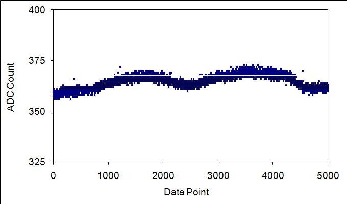
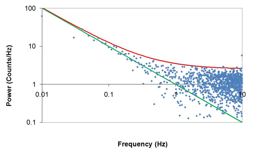
The green line in the spectrum is for a fall-off in noise of 1/f, that is, thermal drift. The total noise asymptote, the red line, sums 2.5 counts (RMS) per decade of frequency white noise with the 1/f noise. This is the same as saying that above 1 Hz, the 16 bit converter is operating at 13.5 effective bits (13.5 effective + 2.5 noise = 16), and below 1 Hz, the drift in the overall measurement system results in higher noise.

Full scale range

What range of signals needs to be recorded? The electrical power grid may carry 60 kV at 120 kA, while a biological cell may have ion currents ~ fA at potential to a few μV. ADC boards typically have full scale ranges no bigger than ±15 V, but may have uni- or bipolar settings and ranges as low as 10 mV. The number of bits one needs interacts with the range. Suppose a measurement is needed with a resolution of 10 μV. To ensure that one can see noise on top of this range, one least significant bit might need to be 1 μV. If one were using a unipolar ADC, at 12 bits full scale would have to be 2¹² * 1 μV = 4.096 mV, a most unlikely combination. At 16 bits, full scale would be
2¹⁶ * 1 μV = 65.54 mV, still smaller than is common, but conceivable. But for a 24 bit converter, full scale would be 2²⁴ * 1 μV = 16.77 V, bigger than any common range. So a real 24 bit converter would be used on the ±5 V range, with a least significant bit magnitude of about 10 V/2²⁴ = 0.6 μV.

Differential vs. single-ended

To what is a potential measurement referenced? Think of a battery you hold in your hand. The difference in potential across the battery is 1.5 V or 9 V or whatever its rating may be. But which end is 0? NEITHER! Either end can be DEFINED to be zero, but neither end is inherently the zero reference! Typically, one defines zero as the potential of the watertable underlying the structure in which an experiment is performed. Most ADCs allow the user to select whether the defined/ground connection from the wall plug is the measurement reference (single-ended input), or if the difference between the high and low sides of a potential difference are to be measured independent of the wall ground (double-ended or differential input). Typically, ADC cards are wired such that one can measure twice as many single-ended as differential inputs. Because common mode noise (noise that effects both the signal to be measured and the reference against which it is measured) is common (for example, from power line noise), differential input is usually quieter than single-ended.

Communications interface

All through these modules, we have regarded digitization as an end in itself. Of course, digitization is just a step in a measurement process. Following digitization, what happens? One may display the result (for example on an LCD panel). The number may be communicated to a computer serially (USB interface, Bluetooth wireless, Firewire, Serial Peripheral Interface, or RS-232) or in parallel (parallel ports, direct memory access). Coverage of how these interfaces work is beyond the scope of this module, but one must be aware that the data encoding as discussed in Number Representation is of great importance here. Choosing an ADC whose output format matches that of a controlling system saves much labor!