Why Digitize Data?

Before we plunge into how digitization works, it's a good idea to remind ourselves why digitization has become ubiquitous.

End of Noise Addition

Physical quantities are noisy. Light is made up of photons, whose numbers typically vary according to a Poisson Distribution (uncertainty in the number of photons = square root of that number). Volumes, masses, currents, pressures, and temperatures all fluctuate. Every time a signal is transduced from one form to another, noise is added -- until the signal is converted to a number. While there is a small probability that a digital computer will fail or a memory chip wipe out, digitzed data typically is fixed for all time. If the number doesn't change, there's no additional noise. Rule of thumb for the digital age: digitize the signal as close (in space, time, and circuitry) to the point of measurement as possible.

Flexibility of Digital Processing

Once we have data recorded as numbers, we can process it in many ways. Signal averaging? Lock-in amplification? Fourier transformation? Filtering? Taking logarithms or exponentiating? Picking every 17th point? Any of these are simple in a computer, and the various data processing algorithms can all be used on exactly the same numbers. In continuous or quantized physical systems, each data stream can be processed only as it occurs and only in one way. Even if several electronic modules are connected to the same node in instrument, the noise in each module will be slightly different.

Report Convenience

Results can be delivered in a form most convenient for the user rather than in a form most closely linked to the result of signal transduction.

The Flip Side of Digitization: Common Misunderstandings

There are a number of common misconceptions and errors connected with the use of digitized data. We list the most common here. As we have not yet discussed any digitization process, the goal is not (yet!) quantitative understanding of the problems, but rather an intuitive idea of what is going on.

Number of significant figures

Every digitization yields only a specific number of digits. Data processing programs do not necessarily recognize this. For example, suppose that we want to find the signal-to-noise ratio for an intensity measurement, and we digitize the signal to find that the number of photons observed during a measurement interval was 327183. What is the signal-to-noise ratio? We know it should be the square root of the number of photons observed. The calculator application that comes in Microsoft WindowsXP shows that 327183^1/2 = 571.99912587345795698295097687708. Now, really, how can a 6 digit measurement result in an answer with 32 digits of precision? This is absurd. Arithmetically, of course, there's no problem, but since there's uncertainty in the original measurement, most of the digits are only arithmetic eye candy, not physical reality. One might say 327183^1/2 = 572, and that would be defensible. However, that suggests that we know the signal-to-noise ratio to 3 significant figures, that it's 572, not 571 and not 573. That hardly seems credible for a single measurement. Saying S/N = 600 (only one significant figure) or 570 (2 significant figures) is probably better. This is a simple example, but ensuring that we only report significant figures, not arithmetic detritus, is critical.

Aliasing and speed of response

Surf to YouTube and watch the demonstration of a strobe light illuminating a fan. If an event happens 100 times per second and we sample it at 100 Hz, we get what looks like a DC signal -- no change as a function of time. If we sample at 101 Hz, the signal changes through one cycle in one second, or the 100 Hz signal has been "aliased" to 1 Hz. This frequency shifting can be useful (in the case of NMR, where it is rare for signals to be even 0.1% shifted in frequency, a 500 MHz raw signal aliased at 499 MHz allows digitization at 1 MHz). When aliasing occurs and we are unaware of it, we get a false sense of what is happening. Sampling at the power line frequency (50 Hz in most of the world, 60 Hz in North America) aliases away noise from power supplies.

For time-dependent signals, we need to sample the waveform many times to accurately map out the shape of what is happening. Thus, the speed with which a signal changes dictates how rapidly we must digitize.

Interpolation and extrapolation

Suppose you have obtained a set of digital data and plotted a working curve. If you make a fresh measurement on a fresh sample, can you use the working curve to measure the behavior of that sample? Usually, the answer is: if the new data fall within the range of the working curve so that one interpolates, one can trust the new data, but if the new data fall outside the previously validated range, one can not trust the use of the curve. Certainly distrusting extrapolation is appropriate for digitized as well as continuous (analog) data. But is interpolation within the range of a working curve always justified? With sufficient signal averaging so that there are sufficient significant figures, the answer is yes, but for sufficiently low noise systems, the granularity of digitization poses a problem. Since all digitization is inherently an integer process, there will be jumps in the measurement output as the digitized value increments by one count at a time. This is stairstepping.

Stair-stepping

As we vary a continuous variable, typically electrical potential, and digitize the value, we get a response that, in the absence of noise, looks like this:

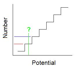
The horizontal red and blue lines show two integer values that can represent potential. If the potential is actually that indicated by the vertical green line, then what? Either the blue or red number will appear, giving no indication that the actual number should be half-way in between!

Only if there is noise, so that the instantaneous value jumps back and forth between the red and blue levels can we signal average to get a fractional number that would allow interpolation!

Discussion Question

The output from a digitizer is the following set of numbers:

2343
2343
2342
2343
2343

Is there a way to tell if the true value is 2343, with a noise spike giving 2342 or a true value of 2342.8? Instructor's thoughts.