iv) Additional considerations in cyclic voltammetry

1) Capacitive Current

As discussed previously, a change in the applied potential of the working electrode will always be accompanied by a rearrangement of the ions in the double layer, leading to a contribution to the signal at each potential from capacitive current. In the CV experiment, a capacitive current “envelope” can be obtained when the scan is done in the electrolyte solution containing no faradaic species. The size of the capacitive current contribution is a function of several things, including the area of the electrode and the scan rate. In many cases, it is much smaller than the faradaic component, and can be effectively ignored. When necessary, it is possible to record the background scan and digitally subtract it from the scan collected for the solution of interest. For most electrode materials, the capacitance ranges from 10 – 40 μF/cm².² In Figure 27, the same conditions were used as in Figure 18 except that a capacitive component (C_DL) equivalent to 40 μF/cm² has been added. The current – potential profile recorded in electrolyte solution only is shown as the blue trace. The red trace shows the CV scan for a 1.0 mM solution of redox active material in the same electrolyte with the same capacitive component included. (DigiElch simulation parameters: v = 0.10 V/s; A = 0.050 cm²; C_i = 1.0 mol/cm³; D = 1.0 x 10^-5 cm²/s; α = 0.50; k_s = 100 cm/s; C_DL = 40 μF/cm²)

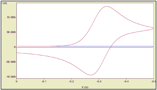
Figure 27

Note that under the conditions of Figure 27, the charging current contributes very little to the cyclic voltammogram. Under different conditions, however, the C_DL can be quite significant. Shown in Figure 28 are two cyclic voltammograms (CVs) for which only one simulation condition was changed for each from those used to produce Figure 27. At left, the concentration of electroactive species was reduced from 1.0 mol/cm³ to 0.05 mol/cm³. At right, the scan rate was increased from 0.10 V/s to 100 V/s. Each change brought about an enhancement of the observed charging current relative to the faradaic current. It should be noted that high scan rates like that used in Figure 27, right are not routinely employed with conventionally-sized electrodes, but work quite well at ultramicroelectrodes, discussed in a separate section.

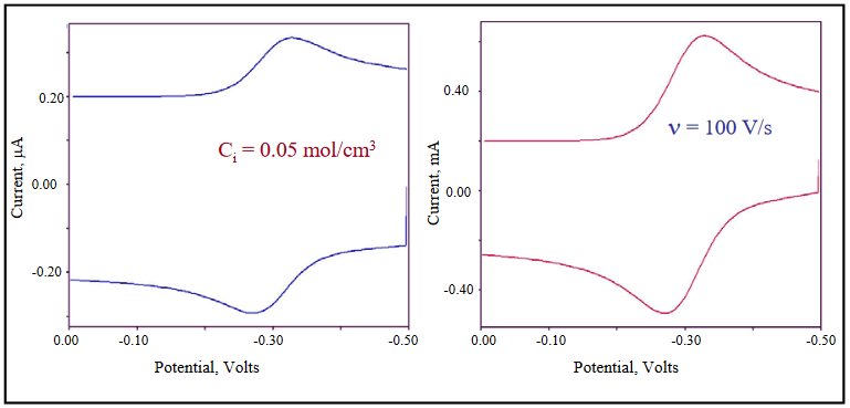
Figure 28

(left: C_i = 0.05 mol/cm³, ν = 0.10 V/s; right: C_i = 1.0 mol/cm³, ν = 100 V/s)

2) Solution Resistance

An additional factor that must be considered in the application of sweep voltammetric methods is that of solution resistance. In a normal three-electrode cell, the potential of the working electrode (WE) is maintained at the desired level relative to the reference electrode (RE) by a device called a potentiostat. We have seen how changing the applied potential, E_a, at the WE allows us to do work in the form of oxidation or reduction of a solution species in the vicinity of the E⁰’ for the redox pair. Since current must pass in the cell to accomplish this work, the resistance of the solution to charge movement (i.e., current) will be responsible for a potential drop between the electrodes in the cell, called the Ohmic drop. The magnitude of the Ohmic drop, E_iR, is given by Ohm’s Law

\[\mathrm{E_{iR} = i_{cell}\: R_s}\]

where i_cell is the current flowing in the cell, and R_s is the solution resistance. In essence, the potential observed by a solution species at the WE is now lower in magnitude than that indicated by the potential measuring device.

The solution resistance is composed of two components in the three electrode cell: that between the auxiliary electrode (AE) and the reference electrode, designated R_c, and that between the reference electrode and the working electrode, R_u. R_c and R_u refer to compensated and uncompensated resistance, respectively. By design, the three electrode potentiostat uses negative electronic feedback between the AE and the RE to “compensate” for the potential drop between those two electrodes, essentially adding in extra potential equal to i_cellR_c to that being applied at the WE. The potential drop between the WE and the RE is not compensated directly by the potentiostat. In most applications, proper location of the RE tip near the WE, many times by use of a Luggin capillary, can minimize the effect of i_cellR_u on the applied potential. In addition, some commercial instruments are available with hardware and software capabilities designed to reduce or eliminate R_u.

Effects of uncompensated resistance are most evident under conditions resulting in large amplitude currents (high concentrations, large electrode area, fast scan rates) or involving low dielectric solvents (many organic). A general observation for voltammetry is that current – potential curves tend to be drawn out over extended potential ranges. In cyclic voltammetry, values for ∆E_p, the separation between the forward and reverse peak potentials, are increased over theoretical values. Peak currents are also reduced below those predicted for reversible systems by the Randles – Sevcik equation. Similar effects are also seen for slow rates of heterogeneous electron transfer, and one must take care to differentiate between the causes. Increases in ∆E_p with scan rate which result from slow kinetics will remain the same for differing concentrations of the analyte of interest, while the effect will be decreased for lower concentration if the result of solution resistance.¹⁴

Figure 29 shows the drawing out of CV waves resulting from uncompensated solution resistance as the scan rate increases. Uncompensated resistance was simulated at 100 Ω. Other parameters were: A = 0.050 cm²; C_i = 1.0 mol/cm³; D = 1.0 x 10^-5 cm²/s; α = 0.50; k_s = 100 cm/s. The expected value of ∆E_p for an uncomplicated, reversible electron transfer is 59/n mV.

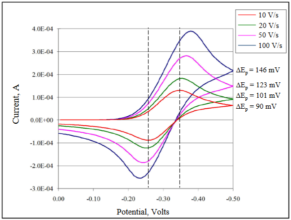
Figure 29